Lab 8: Variational Inference vs HMC#
This lab is adapted from AM207 (Harvard). Data files are in the book’s data/ folder. Worked solutions are collapsed: try each exercise before expanding them.
Problem Description: Compare HMC and Variational Inference for Difficult Posteriors#
In this lab, we will study how HMC and variational inference can struggle with difficult posteriors.
As an inspiration, check out the likelihood (and posterior) landscapes of Bayesian Neural Networks (BNNs) at:
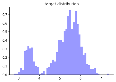
Using the sample code provided below, build up complex distributions with multiple well separated modes as well as multiple modes that blend by defining them as mixtures of Gaussians (see how mixtures of Gaussians are helpful for modeling complex densities!).
Compare how well HMC and variational inference can capture your target distribution. Are there any adjustments to the design choices of the sampler and or VI algorithm that can improve performance (in order to really play around with the settings of HMC and BBVI you’ll need to use your own implementation - pymc3’s implementations have limited allowance for user adjustment)?
def plot_gaussian_mixture(w, mu, sd, S=100):
    '''function for sampling form a mixture of gaussians'''
    K = len(w)
    components = np.random.choice(np.arange(K), replace=True, p=w, size=S)
    samples = [np.random.normal(mu[z], sd[z]) for z in components]
    return samples
#mixture weights
w = pm.floatX([.2, .8])
#mixture means
mu = pm.floatX([3.5, 5.5])
#mixture standard deviations
sd = pm.floatX([.2, .5])

#sample from the mixture and visualize
samples = plot_gaussian_mixture(w, mu, sd, S=1000)
plt.hist(samples, density=True, bins=50, color='blue', alpha=0.4)
plt.title('target distribution')
plt.show()
Solution
The saved outputs below come from the first model (a Bayesian logistic regression with a single observation), not from the Gaussian mixture: when the notebook was run, the mixture cell failed because it did not import theano. Re-running them requires pymc3.
#define a Bayesian logistic regression model in pymc3 (the saved outputs below come from it)
with pm.Model() as model:
    w = pm.Normal('w', mu=0, sd=1)
    theta = pm.math.sigmoid(-20 * w + 10)
    y_1 = pm.Bernoulli('y_1', p=theta, observed=1)
#define the mixture model in pymc3
import theano
with pm.Model() as model:
    x = pm.NormalMixture('x', w=w, mu=mu, sigma=sd, dtype=theano.config.floatX)
#sample from the model using No-U-turn HMC
with model:
    trace = pm.sample(5000)
#check the traceplot for convergence
pm.traceplot(trace)
plt.show()

#approximate the target distribution using variational inference
with model:
    mean_field = pm.ADVI()
    mean_field.fit(n=10000, callbacks=[pm.callbacks.CheckParametersConvergence(every=100, diff='absolute', tolerance=1e-4)])
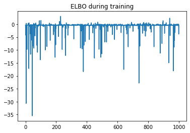
#plot the ELBO
plt.plot(-mean_field.hist[::10])
plt.title('ELBO during training')
plt.show()
#visualize variational posterior
plt.hist(mean_field.approx.sample(1000)['w'], bins=50, color='LightSeaGreen')
plt.title('variational approximation of target distribution')
plt.show()
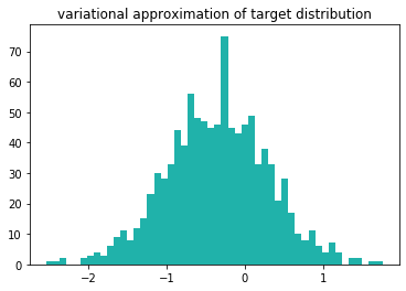
mean_field.approx.sample(1000)['w'].mean()
-0.3545650265571895
mean_field.approx.sample(1000)['w'].std()
0.6606441067212657
Not covered here: a comparison of how well HMC and variational inference capture the target distribution.