Sampling for Posterior Simulation

6. Sampling for Posterior Simulation#

This chapter is adapted from AM207 (Harvard, Fall 2021). Watch the recorded lecture.

In this chapter

Basics of Sampling
Inverse CDF Sampling
Rejection Sampling
Gibbs Sampling

6.1. Basics of Sampling#

Motivation#

Note that nearly every computation for Bayesian models requires us being able to obtain samples from the posterior:

Generating synthetic data from the posterior predictive require us to sample from the model parameters from the posterior, and then sample data given each of these parameters samples.
Empirically computing the posterior predictive mean requires samples from the posterior.
Evaluating the fit of the Bayesian model, i.e. empirically computing the marginal data log-likelihood, requires us to average the likelihood of the data over parameter samples from the posterior.

This is why Bayesian inference relies crucially on the tractability of the posterior. And yet, the posterior of most Bayesian models do not have nice simple closed forms! So how to we sample from these posteriors?

What is Sampling?#

Given a distribution $p(x)$ over a space $\mathbb{R}^D$, sampling $x \sim p(x)$ means to generate a random $x\in \mathbb{R}^D$, such that the asymptotic frequencies of the samples generated is described by the pdf $p(x)$.

A sampler is an algorithm or procedure that produces numbers with a certain distribution $p(x)$.

In practice, “random numbers” are simulated using deterministic algorithms called pseudo number generators. A pseudo number generator takes an initial value, the random seed, and produces an array of random looking numbers (from a uniform distribution).

Note: for a given pseudo number generator, if the random seed is fixed then the random number output will also be fixed.

Simulating a Uniform Random Variable: Linear Congruence#

Fix an integer $c > N$ and fix integers $a, b > 0$.

seed: set an integer $0\leq s_0 < c$
iterate $N$ times:

\[s_n = (as_{n-1} + b)_{\text{mod } c}\]

Output is an array of random integers $[s_0, \ldots, s_N]$ in $[0, c]$.

For an array of random real numbers in $[0, 1]$, we compute $\left[\frac{s_0}{c}, \ldots, \frac{s_N}{c}\right]$.

We’ll see that the simulation of all random variables is based on the simulation of the uniform distribution over $[0, 1]$!

Note: the apparent randomness of the output is sensitive to choices of $a, b, c$.

#parameters of linear congruence algorithm
c = 100
a = 11
b = 5
#total number of simulations
N = 10
#random seed
s_current = 3
#array of random numbers
random_numbers = []

#run the linear congruence algorithm N times
for n in range(N):
    s_next = (a * s_current + b) % c
    random_numbers.append(s_next)
    s_current = s_next
    
#convert random integers to random real values in [0, 1]    
random_numbers = np.array(random_numbers) * 1.
random_numbers /= c
#print
random_numbers

array([0.38, 0.23, 0.58, 0.43, 0.78, 0.63, 0.98, 0.83, 0.18, 0.03])

6.2. Inverse CDF Sampling#

The Cumulative Distribution Function#

Recall that the cumulative distribution function (CDF) of a real-valued random variable $X$ with continuous pdf $f_X$ is defined as

\[ F_X(a) = \mathbb{P}[X \leq a] = \int_{-\infty}^a f_X(t) dt \]

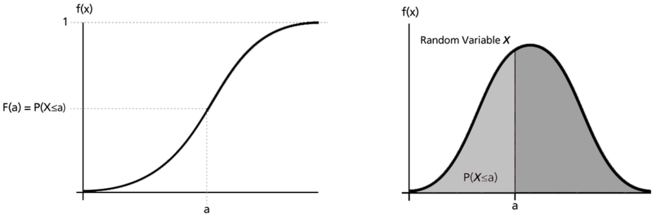
Inverse CDF Sampling: An Intuition#

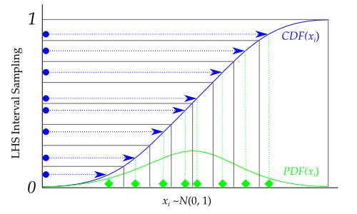
The idea behind Inverse CDF Sampling is that while it is sometimes difficult to generate values for $X$ with the relative frequency described by pdf, $f_X$, it can be easier to generate values for $X$ using the CDF.

The intuition is as follows:

While the support of the pdf and CDF can be unbounded, the range of the CDF is bounded between 0 and 1.
The CDF for a continuous single-variable pdf is an invertible function (on the support of the pdf). That is, each value between 0 and 1 corresponds to a unique value of the random variable $X$.
Values of $X$ that lie under peaks of the pdf occupy larger portions of the interval [0, 1]. That is, the range of the CDF, [0, 1], can be subdivided to exactly reflect the areas of high probability mass and low probability mass under the pdf.

So if we uniformly sample values in the range of the CDF, [0, 1] and find the corresponding $X$ values for these samples (using the inverse function of the CDF), we obtain samples of $X$.

Inverse CDF Sampling: Algorithm#

We use a random variable $U$ with uniform distribution over $[0, 1]$ to simulate a univariate random variable $X$ with pdf $f_X$, where:

we know the analytical form of the CDF of $X$, $F_X$.
we know the analytical form of the inverse of the CDF of $X$, $F^{-1}_X$.

To simulate $X$, we repeat for $N$ number of samples:

sample

\[U_n \sim U(0, 1)\]
compute

\[X_n = F^{-1}_X(U_n)\]

Question: How do we simulate multivariate random variables? What if we don’t have the analytical form of $F^{-1}_X$?

Inverse CDF Sampling: Proof of Correctness#

Theorem: Let $F_X$ be the continuous and strictly increasing CDF of a real-valued random variable $X$. Let $F_X^{−1} : [0,1] \to \mathbb{R}$ be the inverse function of $F_X$. Let $U \sim U(0,1)$, then the random variable $Y = F_X^{−1}(U)$ has CDF $F_X$.

Proof: Recall that the CDF of $Y$ is defined by $F_Y(x) = \mathbb{P}[Y \leq x]$. Now, we can write

\[\begin{split}\begin{aligned} F_Y(x) &= \mathbb{P}[Y \leq x]&\\ &= \mathbb{P}[F_X^{−1}(U) \leq x],&(\text{since $Y = F_X(U)$})\\ &= \mathbb{P}[F_X(F_X^{−1}(U)) \leq F_X(x)],&(\text{since $F_X$ is strictly increasing})\\ &= \mathbb{P}[U \leq F_X(x)],&(\text{since $F_X^{-1}$ is the inverse of $F_X$})\\ &= F_X(x)& (\text{since $0\leq F_X\leq 1$}) \end{aligned}\end{split}\]

Simulating an Exponential Random Variable#

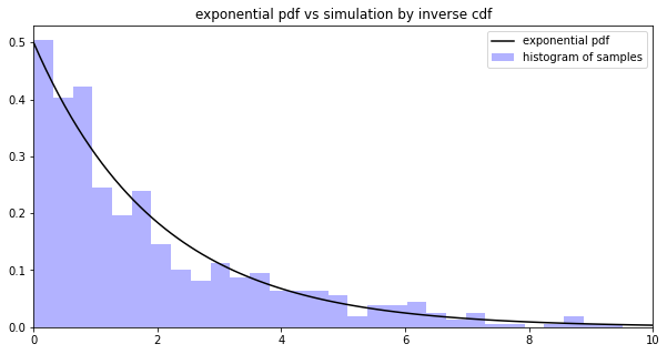
We’ll use a uniform random variable $U\sim U(0, 1)$ to simulate a exponential variable $X\sim Exp(\lambda)$. Recall that the exponential CDF is

\[ F_X(x) = 1 - e^{-\lambda x}. \]

The inverse of the CDF can be found by solving for the input, $x$, of the CDF

\[\begin{split}\begin{aligned} y &= 1 - e^{-\lambda x}\\ e^{-\lambda x} &= 1 - y\\ -\lambda x &= \log(1 - y)\\ x &= -\frac{1}{\lambda}\log(1 - y) \end{aligned}\end{split}\]

where we take $\log$ to be base $e$.

Thus, $F_X^{-1}(y) = -\frac{1}{\lambda}\log(1 - y)$.

#plot true pdf and samples
fig, ax = plt.subplots(1, 1, figsize=(10, 5))
x = np.linspace(0, 10, 100)
ax.plot(x, exp_pmf(x), color='black', label='exponential pdf')
ax.hist(samples, bins=50, density=True, color='blue', alpha=0.3, label='histogram of samples')
ax.set_title('exponential pdf vs simulation by inverse cdf')
ax.set_xlim([0, 10])
ax.legend(loc='best')
plt.show()   

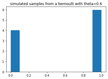
../_images/dcef890a69fea211bf682063947f67f350a9c8ce8eab319f2c657f14c76833b9.png

Simulating a Bernoulli Random Variable#

The CDF of a discrete random variable $X$ with $K$ possible outputs is a step function:

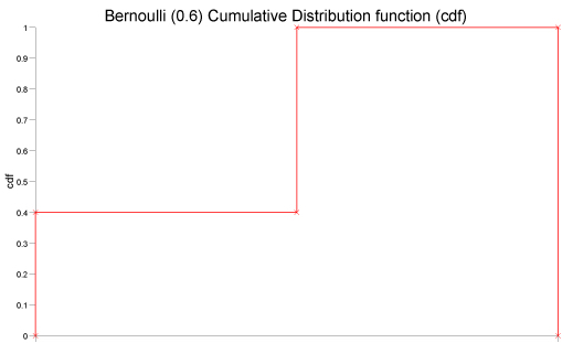
Technically this CDF is not invertible. But we can easily map the output of the CDF to values of $X$. The CDF naturally divides the interval [0, 1] into $K$ parts, each part should be mapped to a case where $X=k$. For example, the Bernoulli CDF divides up the interval into two parts, the first $[0, 1-\theta]$ maps to naturally to $X=0$ and the second $[0, 1-\theta]$ maps to $X=1$.

Thus, to simulate a Bernoulli random variable $X \sim Ber(\theta)$, we

sample $U\sim U(0, 1)$
if $U<1-\theta$ we map to $X=0$, otherwise we map to $X=1$

This process is easily extended to categorical variables with $K$ categories.

#plot samples
plt.hist(u, density=True)
plt.title('simulated samples from a bernoulli with theta={}'.format(theta))
plt.show()    

../_images/79528ee471e54b790977023bf7bda37e830770826fb689dff10a8c660a0f7239.png

What Can We Simulate?#

We can simulate sampling from univariate continuous distributions with closed form inverse CDF’s, e.g. exponential random variables. We can’t simulate normal random variables since the normal CDF does not have a closed form inverse! We can’t simulate multivariate random variables.

We can simulate discrete random variables.

6.3. Rejection Sampling#

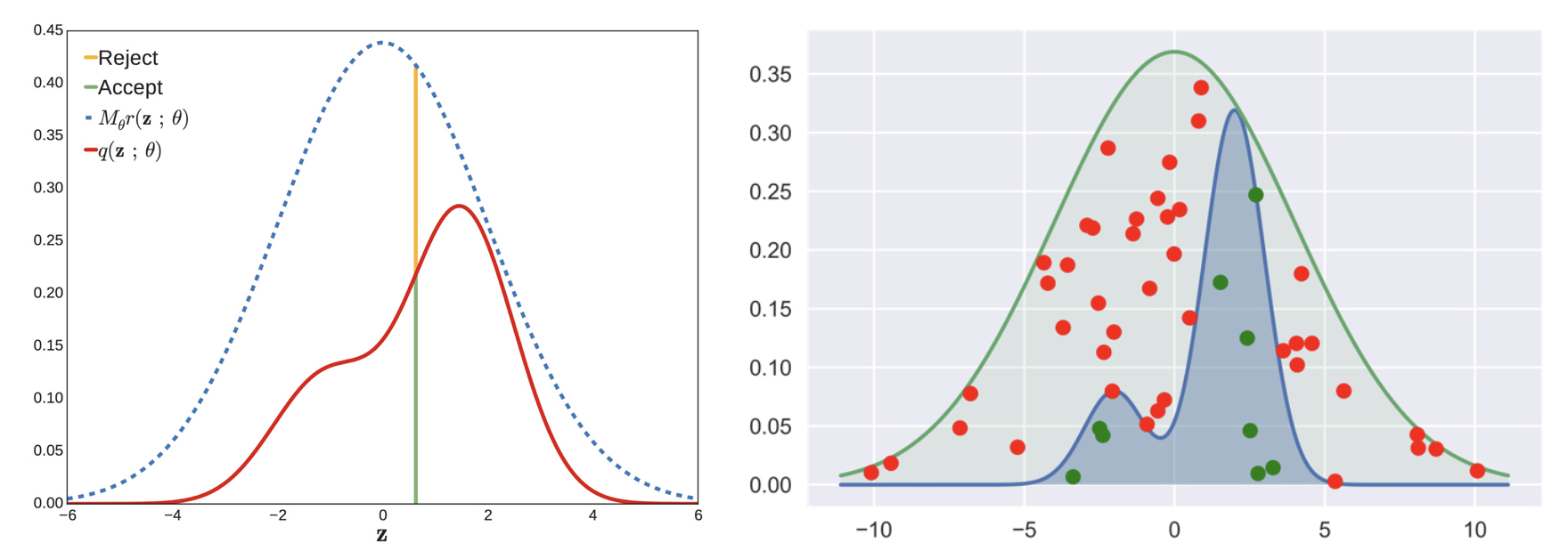
Rejection Sampling: An Intuition#

The idea behind Rejection Sampling is to by-pass the problem of sampling from a difficult distribution $f_X$, by:

approximating $f_X$ (called the target distribution), with a pdf $g$ (called the proposal distribution) that is easy to sample
sample from $g$ and reject the samples that are unlikely to be from $f_X$

Rejection Sampling: Algorithm#

We can use rejection sampling to simulate multivariate random variables and random variables for which we don’t have a closed form for $F^{-1}_X$. We choose a proposal distribution $g$ such that (1) the support of $g$ covers the support of $f$ and (2) there is a constant $M > 0$ with $\frac{f_X(y)}{g(y)} \leq M$ for all $y$.

In less high-falutin talk: we need (1) $g$ to be non-zero where ever $f$ is and $g$ must decay slower than $f$ (2) M * g is an upper bound of $f$.

To simulate $X$, we repeat until $N$ samples are accepted:

sample $Y_k \sim g(Y)$
sample a random height, $U_k \sim U(0, 1)$
if $U_k < \frac{f_X(Y_k)}{Mg(Y_k)}$ then accept $Y_k$ as a sample, else reject

Question: How long does it take to accumulate $N$ samples? What is the effect of the choice of the proposal distribution $g$ have on the sampling process? Now that we can sample from any distribution, we’re done, right?

Going deeper: Rejection Sampling: Proof of Correctness

We need to show that the accepted samples $Y$ have same distribution as $X$. In particular, we’ll show that the CDF of the accepted samples is equal to $F_X$:

\[ \mathbb{P}\left[ Y \leq a\; \left\vert\; U \leq \frac{f_X(Y)}{Mg(Y)}\right. \right] = F_X(a). \]

Using Bayes’ rule for probabilities, we get that

\[\begin{split}\begin{aligned} \mathbb{P}\left[\left.U \leq \frac{f_X(Y)}{Mg(Y)} \; \right\vert\; Y \leq a \right] &= \frac{\mathbb{P}\left[Y \leq a,\; U \leq \frac{f_X(Y)}{Mg(Y)} \right]}{\mathbb{P}\left[ Y \leq a\right]}\\ &= \int_{-\infty}^a \frac{\mathbb{P}\left[\left.U \leq \frac{f_X(Y)}{Mg(Y)} \; \right\vert\; Y \leq y \leq a \right] g(y)}{\mathbb{P}\left[ Y \leq a\right]} dy\\ &= \frac{1}{\mathbb{P}\left[ Y \leq a\right]}\int_{-\infty}^a \mathbb{P}\left[\left.U \leq \frac{f_X(Y)}{Mg(Y)} \; \right\vert\; Y \leq y \leq a \right] g(y) dy\\ &= \frac{1}{\mathbb{P}\left[ Y \leq a\right]} \int_{-\infty}^a \frac{f_X(y)}{Mg(y)} g(y) dy\\ &= \frac{1}{M\mathbb{P}\left[ Y \leq a\right]} \int_{-\infty}^a f_X(y) dy\\ &= \frac{1}{M\mathbb{P}\left[ Y \leq a\right]} \mathbb{P}\left[ X \leq a\right]\\ &= \frac{F_X(a)}{MG(a)} \end{aligned}\end{split}\]

where $G$ is the CDF of the proposal pdf $g$.

Now, we can write:

\[\begin{split}\begin{aligned} \mathbb{P}\left[ Y \leq a\; \left\vert\; U \leq \frac{f_X(Y)}{Mg(Y)}\right. \right] &= \frac{\mathbb{P}\left[\left.U \leq \frac{f_X(Y)}{Mg(Y)} \; \right\vert\; Y \leq a \right] \mathbb{P}\left[ Y \leq a\right]}{\mathbb{P}\left[U \leq \frac{f_X(Y)}{Mg(Y)}\right]}\\ &= \frac{\frac{F_X(a)}{MG(a)} * G(a)}{1/M}\\ &= F_X(a) \end{aligned}\end{split}\]

which is exactly what we wanted to show.

Rejection Sampling: Efficiency#

Given a proposal $Y=y$, the probability of accepting it is

\[ \mathbb{P}\left[\left.U\leq \frac{f(Y)}{Mg(Y)} \right\vert Y=y\right] = \frac{f(y)}{Mg(y)}. \]

So the overall probability $p$ of accepting any given proposal can be computed by integrating out $y$:

\[\begin{split}\begin{aligned} p &= \int_{\mathbb{R}} \frac{f(y)}{Mg(y)} g(y)dy \\ &= \frac{1}{M} \int_{\mathbb{R}} f(y) dy\\ &= \frac{1}{M} \end{aligned}\end{split}\]

We see that the expected number of times it takes to draw and accept a sample $X=x$ is precisely $M$. This means that roughly $(M-1)/M$ of samples drawn from $g$ will be rejected. When $M$ is large, the rejection sampler is very inefficient.

Simulating a Normal Random Variable#

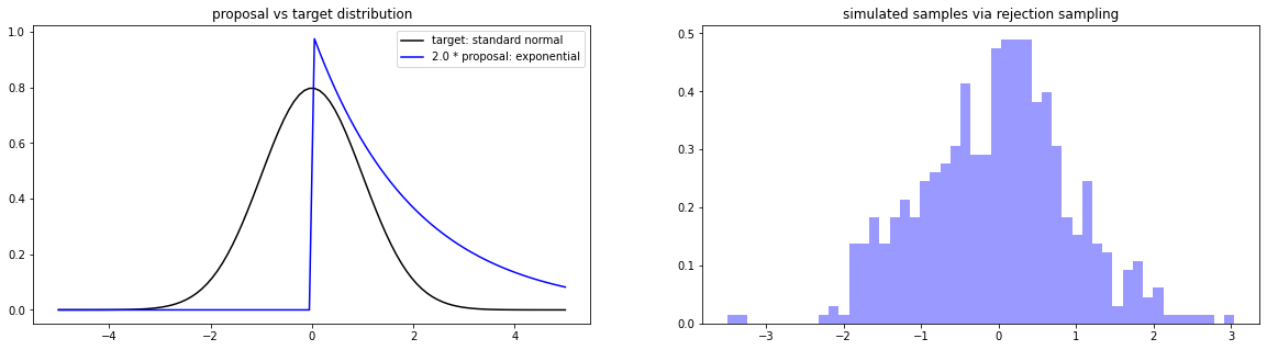
We note that if we can simulate a standard normal variable $X\sim \mathcal{N}(0, 1)$, then we can simulate any normal variable $Y\sim \mathcal{N}(\mu, \sigma^2)$ by setting $Y = \sigma* X + \mu$.

We also observe that since the standard normal distribution is symmetric about $X=0$, we only need to simulate samples from the non-negative side of $\mathcal{N}(0, 1)$ and then independently sample a sign (+ or -) for each sample using a Bernoulli distribution with $\theta = 0.5$.

Simulating the positive half of the normal distribution means we need to scale the normal pdf by a factor of 2, so that is integrates to 1 over the nonnegative real numbers.

A natural candidate for a pdf to cover the non-negative half of the standard normal pdf is the exponential pdf.

#plot samples
fig, ax = plt.subplots(1, 2, figsize=(20, 5))
x = np.linspace(-5, 5, 100)
ax[0].plot(x, 2 * target_pdf(x), color='black', label='target: standard normal')
ax[0].plot(x, M * proposal_pdf(x), color='blue', label='{} * proposal: exponential'.format(M))
ax[0].set_title('proposal vs target distribution')
ax[0].legend(loc='best')
ax[1].hist(samples, bins=50, density=True, color='blue', alpha=0.4)
ax[1].set_title('simulated samples via rejection sampling')
plt.show()   

../_images/0253075bd7bef95a37dcfed165f8dd2de2524221d4c347418f957536722d4ef6.png

What Can We Simulate?#

We can simulate any continuous or discrete random variable as long as we can find a suitable proposal distribution.

But as the dimensions of the random variable increases or for inappropriate choices of the proposal distribution, the efficiency of this sampler may be very low.

Limitations of Rejection Sampling in High Dimensions#

Since the acceptance rate for rejection sampling is 1/M, where $M$ is a constant that bounds $\frac{f_X(y)}{g(y)}$ for all $y$, we’d want to make $M$ as close to $1$ as possible, i.e. we want $g(y)$ to be approximately equal to $f_X(y)$. In general this is very difficult to achieve, especially in high dimensions.

Example:

Let’s say our target distribution is a $D$-dimensional Gaussian $\mathcal{N}\left(0, \sigma_f^2\mathbf{I}_{D\times D}\right)$, where $\mathbf{I}_{D\times D}$ is a $D\times D$ identity matrix. Let’s fix the proposal distribution to be a $D$-dimensional Gaussian $\mathcal{N}\left(0, \sigma_g^2\mathbf{I}_{D\times D}\right)$, where $\sigma_g > \sigma_f$. We can compute the optimum value of $M$ to be $\left(\frac{\sigma_g}{\sigma_f}\right)^D$. But this is a value that scales with $D$! For example, if $D=1,000$ and $\frac{\sigma_g}{\sigma_f} = 1.01$ then the probability of accepting a sample will be $\frac{1}{M} = 0.000047$.

6.4. Gibbs Sampling#

Semi-Conjugate Priors#

Let $Y \sim \mathcal{N}(\mu, \sigma^2)$, with both parameters unknown. We place a normal prior on $\mu$, $\mu\sim\mathcal{N}(m, s^2)$, and an gamma prior on $\sigma^2$, $\sigma^2\sim IG(\alpha, \beta)$.

The posterior $p(\mu, \sigma^2|Y)$ is then:

\[\begin{aligned} p(\mu, \sigma^2 | Y) = \frac{\overbrace{\frac{1}{\sqrt{2\pi \sigma^2}} \mathrm{exp} \left\{-\frac{(Y - \mu)^2}{2\sigma^2}\right\}}^{\text{likelihood}} \overbrace{\frac{1}{\sqrt{2\pi s^2}} \mathrm{exp} \left\{-\frac{(m - \mu)^2}{2s^2}\right\}}^{\text{prior on $\mu$}}\overbrace{\frac{\beta^\alpha}{\Gamma(\alpha)} \left( \sigma^2\right)^{-\alpha -1}\mathrm{exp} \left\{-\frac{\beta}{\sigma^2}\right\}}^{\text{prior on $\sigma^2$}}}{p(Y)} \end{aligned}\]

Note that:

if we condition on $\sigma^2$ (i.e. hold it constant) then $p(\mu| Y, \sigma^2)$ is a normal pdf, $\mathcal{N}\left(\mu; \frac{s^2y + \sigma^2m}{s^2 + \sigma^2}, s^2\sigma^2\right)$.
if we condition on $\mu$ (i.e. hold it constant) then $p(\sigma^2| Y, \mu)$ is an inverse gamma pdf, $IG\left(\sigma^2; \alpha + 0.5, \frac{(y-\mu)^2}{2} + \beta\right)$

That is, the conditional of the posterior are easy to sample from while the joint posterior is not. In this case, we call the priors semi-conjugate for our likelihood.

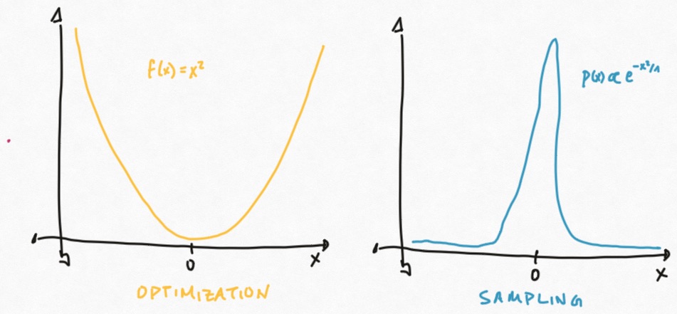
Gibbs Sampling: An Intuition#

If we start at a point $(x^{(0)}, y^{(0)})$ sampled from from the joint distribution $p(X, Y)$, we can get to the next point $(x^{(1)}, y^{(1)}) \sim p(X, Y)$ through a “stepping-stone” $(x^{(1)}, y^{(0)})$, where we updated the first coordinate by $x^{(1)} \sim p(X|Y = y^{(0)})$. From there, we update the second coordinate $y^{(1)} \sim p(Y|X = x^{(1)})$.

The initial samples may be unlikely under $p(X, Y)$, but this process will eventually lead us to a high density area in $p(X, Y)$ and we will mostly sample there.

Gibbs Sampling: Algorithm#

To simulate $N$ samples of a $D$-dimensional multivariate random variable $X$ with pdf $f_X$, we

initialization: choose any $x^{(0)} = \left[x^{(0)}_1\;\; \ldots\;\; x^{(0)}_D\right]$
iterate $N$ times: sample $x^{(n+1)} = \left[x^{(n+1)}_1\;\; \ldots\;\; x^{(n+1)}_D\right]$ by

a. initialization: sample $X^{(n+1)}_1$ from the conditional distribution

\[f_X\left(X_1 \,|\, X_2 = x^{(n)}_2,\;\ldots,\; X_D = x^{(n)}_D\right)\]

b. iterate from $d = 2$ through $d=D$: sample $x^{(n+1)}_d$ from the conditional distribution

\[f_X\left(X_d \,|\, X_1 = x^{(n+1)}_1,\; \ldots,\; X_{d-1} = x^{(n+1)}_{d-1},\; X_{d+1} = x^{(n)}_{d+1},\; \ldots,\; X_D = x^{(n)}_D\right)\]

Claim: When $N$ is large enough, the latter portion of the samples we obtain will be from the distribution of $X$.

Question: Why is this algorithm a valid sampler? That is, how do we prove that the samples we obtain are actually distributed as $f_X$? What is the effect of the initialization $x^{(0)}$?

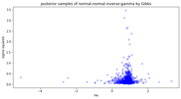
Simulating the Posterior of a Normal-Normal-Inverse Gamma Model#

Let $Y \sim \mathcal{N}(\mu, \sigma^2)$, with both parameters unknown. We place a normal prior on $\mu$, $\mu\sim\mathcal{N}(m, s^2)$, and an gamma prior on $\sigma^2$, $\sigma^2\sim IG(\alpha, \beta)$.

$p(\mu| Y, \sigma^2)$ is a normal pdf,

\[\mathcal{N}\left(\mu; \frac{s^2y + \sigma^2m}{s^2 + \sigma^2}, s^2\sigma^2\right).\]
$p(\sigma^2| Y, \mu)$ is an inverse gamma pdf,

\[IG\left(\sigma^2; \alpha + 0.5, \frac{(y-\mu)^2}{2} + \beta\right).\]

We choose an arbitrary initial point $(\mu_0, \sigma^2_0) \in \mathbb{R}^2$, and then sample the next point by sampling from the conditionals $p(\mu| Y, \sigma^2)$ and $p(\sigma^2| Y, \mu)$, in order.

#plot posterior samples via gibbs
fig, ax = plt.subplots(1, 1, figsize=(10, 5))
x = np.linspace(0, 10, 100)
ax.scatter(posterior_samples[:, 0], posterior_samples[:, 1], color='blue', alpha=0.2)
ax.set_title('posterior samples of normal-normal-inverse-gamma by Gibbs')
ax.set_xlabel('mu')
ax.set_ylabel('sigma squared')
plt.show()   

../_images/28c645a0cd02c60b74187e36d6ca5aac6295a2e90e8b3e91ffe82dfdd4c5e96b.png

6.5. Summarizing Sampling#

Samplers for Simulating Random Variables#

A sampler is a procedure for producing random numbers from a specific distribution $p(X)$. We’ve seen that we can build up samplers for sophisticated distributions, incrementally, starting from a sampler for a uniform distribution $U(0, 1)$.

Linear Congruence Pseudo Random Number Generator: simulates random numbers in $U(0, 1)$. By translating and scaling we can simulate a random variable $U\sim U(a, b)$.
Inverse CDF Sampling: transforms random samples from a uniform distribution $U(0, 1)$ into samples from a univariate distribution $p(X)$ by using the inverse CDF of $X$.
Rejection Sampling: find a proposal distribution $q(X)$ that is (1) easy to sample from and (2) approximates the target distribution $p(X)$. We then sample from $q$ and reject samples that are unlikely under $p$.
Gibbs Sampling: when complex multivariate distributions have easy conditional distributions $p(X_n | X_1, \ldots, X_{n-1}, X_{n+1}, \ldots, X_{N})$, we can obtain samples iteratively by updating the last sample from the conditionals, one coordinate at a time. Eventually, these samples will be from $p(X)$. This allows us to sample from the posterior of models with semi-conjugate priors.

How to Evaluate a Sampler#

Correctness: Every sampler must come with a proof of correctness - that is, the numbers produced by the sampler have the distribution $p(X)$. Many intuitively sensible ways of sampling can fail to be correct.

Question: Why isn’t it sufficient to “histogram” the samples and check that they are distributed like $p(X)$?
Efficiency: Every sampler must be analyzed for it’s efficiency - that is, how many times the procedure must run before it accepts a sample. You should also be aware of how the efficiency is affected by the dimension of $X$.

Question: How do inverse CDF and rejection compare in terms of efficiency?
Sufficiency of repetition: Some samplers like Gibbs comes with the guarantee that if you repeat the procedure enough times (asymptotically), you will eventually be sampling from $p(X)$. But exactly how many times is enough?

Why are We Sampling Again?#

Recall that the primary objects of interest in a Bayesian model are the posterior distribution over parameters and the posterior predictive distribution over observations.

Evaluating the model, forming scientific hypothesis about the data and making predictions all require sampling from one of the two distributions.

When the prior is conjugate for the likelihood, the posterior pdf can be derived in closed form. Often, such a posterior is easy to sample from (using inverse CDF or rejection sampling). However, restricting ourselves to such simple likelihoods and priors limits our ability to model complex real-life data!

Our goal is to develop a set of different procedures that allow us to sample from arbitrary distributions. I.e. samplers will make Bayesian inference more “generic”, less “artisanal”.

What If We Want Posterior Point Estimates?#

Posterior samples allow us to approximately compute posterior point estimates, for example, we can approximate the posterior mean as

\[ \mathbb{E}_{\theta|Y}[\theta] = \int_\Theta \theta\, p(\theta | Y)\,d\theta \approx \frac{1}{S}\sum_{s=1}^S \theta_s,\, \theta_s \sim p(\theta | Y) \]

In fact, for any function $f$ of $\theta | Y$, we can estimate the expected value of $f$ by first sampling $S$ samples from the posterior $p(\theta | Y)$ and then compute the average value of $f$ on these samples:

\[ \mathbb{E}_{\theta|Y}[f(\theta)] = \int_\Theta f(\theta)\, p(\theta | Y)\,d\theta \approx \frac{1}{S}\sum_{s=1}^S f(\theta_s),\, \theta_s \sim p(\theta | Y) \]

Question: But is this estimate consistent? Unbiased? Of minimal variance?

6.6. Summary#

What’s a good strategy for learning/organizing the info in this book?

Every topic is potentially really technical and really deep (e.g. do I need to read a text book on measure-theoretic foundations of probability theory first?), how do you manage diminishing margins of return and your finite energy?
- Ask: what is this good for? Let the tasks and real-life questions guide you to the piece of theory that is necessary to address these tasks/questions productively and responsibly.
- Ask: why do I care? Remember the big-picture story of the book, each topic is linked to the next and builds on the previous. You can Google the details later.
Why Are We Sampling Again? AKA Bayesian Model Evaluation
- (Posterior Predictive Check: Obviously Needs Sampling) Use the models in the posterior to generate synthetic data, in order to compare with real data, i.e. sample from the posterior predictive.
- (Marginal Data Log-Likelihood: Secretly Needs Sampling) Compute the marginal log-likelihood of the data (train or test) over the posterior:
  
  \[\sum_{m=1}^M \log \int_\Theta p(\mathbf{y}^*_m | \theta) p(\theta| \text{Data}) d\theta\]
Why is sampling hard (can’t we numpy.random.something)?
Basic strategy of sampling:
- build up a set of simple distributions that we can pseudo-randomly sample from (e.g. Uniform)
- transform samples from our simple distributions into samples from complex distributions:
  - inverse CDF (only if the CDF is defined can be inverted analytically)
  - rejection sampling (not efficient in high dimensions)
  - Gibbs (only if the conditional distributions are easy to sample from)
How do I evaluate the quality of my samples?
- Can I histogram my samples and compare it with the graph of my target pdf?
- There’s a whole lot of math that came with my sampler, do I need to care?
- Can I customize or change the sampling algorithm?
- If I know that my sampler is correct (e.g. produces actual samples from my target pdf) do I care about any other properties?
But do I REALLY need to be Bayesian???
- Uncertainty is obviously important in many high-impact tasks (e.g. Bayesian Modeling of Uncertainty in Ensembles of Climate Models)
- Even if I ONLY care about prediction, the averaged predictions from an ensemble of models is very often better in terms of accuracy, and Bayesian posteriors naturally given you an ensemble of models. Averaging the predictions of models in the Bayesian posterior is called Bayesian averaging and it can be better in terms of accuracy than even bootstrap ensembles!

6.7. Further Reading#

Sampling

(Introductory) Provable Randomness: How to Test RNGs
(Introductory) Basics of Sampling
(More detailed) How to choose g and M in rejection sampling

Sampling for Posterior Simulation

Contents

6. Sampling for Posterior Simulation#

6.1. Basics of Sampling#

Motivation#

What is Sampling?#

Simulating a Uniform Random Variable: Linear Congruence#

6.2. Inverse CDF Sampling#

The Cumulative Distribution Function#

Inverse CDF Sampling: An Intuition#

Inverse CDF Sampling: Algorithm#

Inverse CDF Sampling: Proof of Correctness#

Simulating an Exponential Random Variable#

Simulating a Bernoulli Random Variable#

What Can We Simulate?#

6.3. Rejection Sampling#

Rejection Sampling: An Intuition#

Rejection Sampling: Algorithm#

Rejection Sampling: Efficiency#

Simulating a Normal Random Variable#

What Can We Simulate?#

Limitations of Rejection Sampling in High Dimensions#

6.4. Gibbs Sampling#

Semi-Conjugate Priors#

Gibbs Sampling: An Intuition#

Gibbs Sampling: Algorithm#

Simulating the Posterior of a Normal-Normal-Inverse Gamma Model#

6.5. Summarizing Sampling#

Samplers for Simulating Random Variables#

How to Evaluate a Sampler#

Why are We Sampling Again?#

What If We Want Posterior Point Estimates?#

6.6. Summary#

6.7. Further Reading#