22. Black-box Variational Inference#
This chapter is adapted from AM207 (Harvard, Fall 2021). Watch the recorded lecture.
In this chapter
Review of Neural Network Models
Bayesian Neural Networks
Black-box Variational Inference
22.1. Review of Neural Network Models#
How Would You Parameterize a Non-linear Trend?#
In non-linear regression, we are interested in modeling observed outcome \(Y^{(n)}\) as a non-linear function of observed covariates \(\mathbf{X}^{(n)}\):
But it’s not easy to think of a function class \(g(x)\) can capture the trend in the data (e.g. polynomial or sinusoidal)?
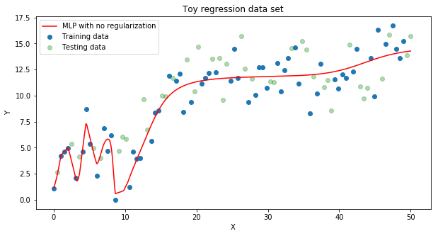
Representing Arbitrarily Complex Functions#
Motto: neural networks build up a complex function \(g\) by composing simple nonlinear functions. We represent neural networks as layered directed graphs where each node \(i\) in the \(l\)-th layer represents the function \(f\left(\sum_{j}w^{l-1}_{ji} h^{l-1}_j\right)\), \(h^{l-1}_j\) being the hidden nodes from the \(l-1\)-th layer.
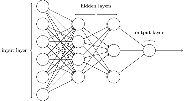
This is a neural network. We denote the weights of the neural network collectively by \(\mathbf{W}\). The non-linear function \(f\) is called the activation function.
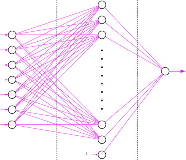
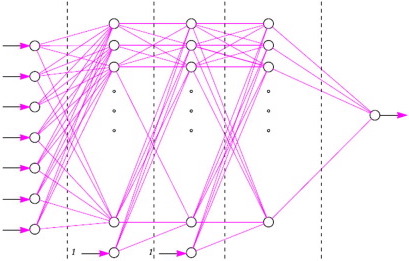
Design Choices: Depth or Width#
Ideally, we want our architecture to be able to express a number of very complex functions, since we don’t know what is appropriate for our data. So what architecture is more effective for expressing complex functions?
|
|
Neural Networks Regression#
Model for Regression: \(Y^{(n)}\sim \mathcal{N}(\mu, \sigma^2)\), \(\mu = g_\mathbf{W}(\mathbf{X}^{(n)})\), where \(g_\mathbf{W}\) is a neural network with parameters \(\mathbf{W}\).
Training Objective: find \(\mathbf{W}\) to maximize the likelihood of our data. This is equivalent to minimizing the Mean Square Error,
Optimizing the Training Objective: The main challenge of optimizing the objective is computing the gradient of a neural network. Luckily, the gradient can be computed in an algorithmic way using the chain rule, working from the output node backwards towards the input. For example, the derivative with respect to the hidden node \(h^l_i\) is:
Using this backwards gradient computation, we can optimize a neural network with respect to the MSE using gradient descent.
The Maximum Likelihood Objective is Non-Convex for Neural Networks#
Unfortunately, the likelihood and MSE functions for neural network regression models are not convex! This means that just because your gradient is zero, it doesn’t mean you’ve optimized anything.
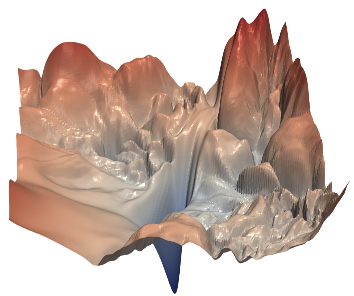
Neural Network Regression vs Linear Regression#
Linear models are easy to interpret. Once we’ve found the MLE of the model parameters, we can formulate scientific hypotheses about the relationship between the outcome \(Y\) and the covariates \(\mathbf{X}\):
What do the weights of a neural network tell you about the relationship between the covariates and the outcome?
Generalization Error and Bias/Variance#
Complex models have low bias – they can model a wide range of functions, given enough samples.
But complex models like neural networks can use their ‘extra’ capacity to explain non-meaningful features of the training data that are unlikely to appear in the test data (i.e. noise). These models have high variance – they are very sensitive to small changes in the data distribution, leading to drastic performance decrease from train to test settings.
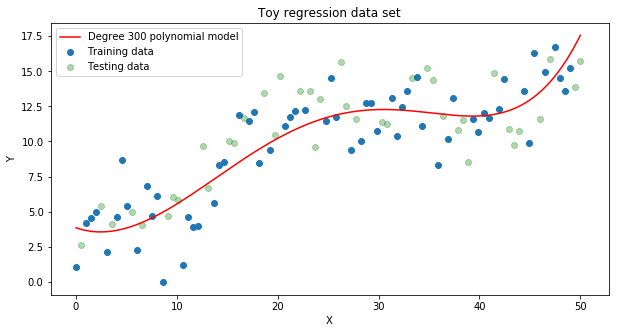
|
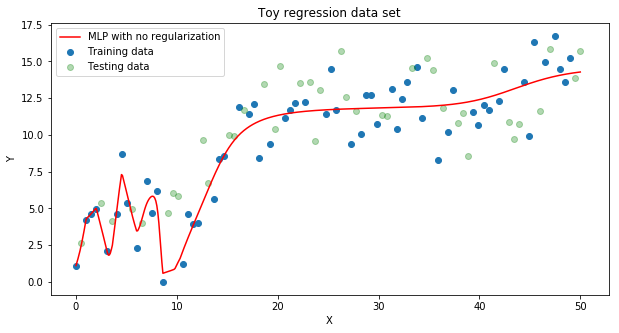
|
22.2. Bayesian Neural Networks#
Bayesian Polynomial Regression is Bayesian Linear Regression#
A Bayesian polynomial regression model uses a polynomial of degree \(D\) to capture the relationship between \(X\in \mathbb{R}\) and \(Y\):
Rather than considering the polynomial as a non-linear function of \(X\), we can see it as a linear function of the vector \(\mathbf{X} = [1, X, X^2, \ldots, X^D] \in \mathbb{R}^{D+1}\):
This means that for a Bayesian polynomial regression model, the posterior \(p(\mathbf{X} | \text{Data})\) is a multivariate Gaussian (just as in the case of Bayesian linear regression, see the Chapter 1 problem set).
Bayesian Neural Networks#
A Bayesian neural network (BNN) is a Bayesian model for regression that uses a neural network to capture the relationship between \(\mathbf{X}\) and \(Y\):
Unfortunately, the posterior of a neural network is multimodal and very complex, posing a challenge for samplers. Furthermore, training data for BNNs are typically large, this makes gradient-based samplers like HMC extremely inefficient – in every leap-frog iteration of HMC, the gradient \(\frac{\partial U(q)}{\partial q}\) requires an evaluation over the entire training data set.
Further reading:
NeuTra-lizing Bad Geometry in Hamiltonian Monte Carlo Using Neural Transport
Stochastic Gradient Hamiltonian Monte Carlo
22.3. Black-box Variational Inference#
Review of Variational Inference#
Goal: given a target posterior distribution \(p(\psi | Y_1, \ldots, Y_N)\), \(\psi \in \mathbb{R}^I\) we want to find a distribution \(q(\psi |\lambda^*)\) in a family of distributions \(Q = \{q(\psi |\lambda) | \lambda \in \Lambda \}\) such that \(q(\psi |\lambda^*)\) best approximates \(p\).
Design Choices: we need to choose:
A. (Variational family) a family \(Q\) of candidate distributions for approximating \(p\). The members of \(Q\) are called the variational distributions.
Our Choice: we assume that the joint \(q(\psi)\) factorizes completely over each dimension of \(\psi\), i.e. \(q(\psi)= \prod_{i=1}^I q(\psi_i | \lambda_i)\). This is called the mean field assumption. What can go wrong with this design choice?
B. (Divergence measure) a divergence measure to quantify the difference between \(p\) and \(q\).
Our Choice:
What can go wrong with this design choice?
Variational Inference as Optimization#
Let’s formalize variational inference for a target distribution \(p(\psi)\): find a \(q(\psi|\lambda^*)\) such that
Recall that for EM, we had proved that minimizing the KL is equivalent to maximizing the ELBO (for which it is easier to compute the gradient). We will do the same here:
Thus, the variational objective can be rephrased as maximizing the \(ELBO\).
Variational Inference for Bayesian Neural Networks#
Consider a Bayesian neural network:
and a mean-field Gaussian variational family:
where \(\Sigma\) is a diagonal matrix.
The ELBO is:
To find the optimal variational parameters such that \(\mu^*, \Sigma^* = \mathrm{argmax}\, ELBO(\mu, \Sigma)\), we need to compute the gradient of the ELBO:
Going deeper: Rewriting the Gradient of the ELBO
To find the optimal variational parameters such that \(\mu^*, \Sigma^* = \mathrm{argmax}\, ELBO(\mu, \Sigma)\), we need to compute the gradient of the ELBO:
The main problem in computing this gradient is that we can’t take the gradient of a complex integral in closed form, and we can’t push the gradient inside the expectation to make the gradient computation easier (since the expectation is over a distribution that involves \(\mu, \Sigma\)). Recall that in Coordinate Ascent Variational Inference (CAVI), we avoided computing this gradient all together, but this required extensive model-specific derivations. In this chapter, we will instead adopt the approach of performing gradient descent taking MC estimates of expectations in the gradient.
But before we estimate the expectation with a sum, we need to push the gradient inside the expectation! To do so, we rewrite the expectation as an integral:
Now, in general, integration and differentiation do not commute meaning \(\nabla \int \neq \int \nabla\). However, in this case, we leverage the properties of the functions inside the integrand to prove that:
Using the product rule, we can differentiate the integrand:
Now, we can do a bit of algebra to break up the integral into pieces and evaluate some easy pieces:
Note that
since \(\nabla_{\mu, \Sigma}\, \log p(\mathbf{W}, \text{Data}) =\mathbf{0}\) because \(p(\mathbf{W}, \text{Data})\) depends neither on \(\mu\) nor \(\Sigma\).
Similarly, we can prove that
The proof is not difficult, it only requires you to write out the gradient for \(\nabla_{\mu, \Sigma}\,\log q(\mathbf{W} | \mu, \Sigma)\),
and then evaluate the expectation as an integral.
Finally, this mean that we are left with:
But the problem is that this doesn’t look like an expectation! So we can’t use MC estimation to approximate this integral! Luckily, we observe the following algebra fact: since we know that \( \nabla_{\mu, \Sigma}\,\log q(\mathbf{W} | \mu, \Sigma) = \frac{\nabla_{\mu, \Sigma}\,q(\mathbf{W} | \mu, \Sigma)}{q(\mathbf{W} | \mu, \Sigma)} \), this gives us
That is, knowing the derivative of the log of a function allows us to compute the gradient of that function! This trick is called the log-derivative trick.
Now, if we replace the gradient of \(q\) in our integral with the gradient of log of \(q\), we get
and this integral can be written as an expectation:
Recombining the two log terms, we get:
That is, we have successfully rewritten the gradient of the ELBO as an expectation of a gradient! The resulting expectation of a gradient is called the score function gradient of the ELBO. Finally, to approximate the gradient, we can perform MC estimation to estimate the expectation and use autograd to compute \( \nabla_{\mu, \Sigma}\, q(\mathbf{W} | \mu, \Sigma)\); and since the gradient is now easily approximated we can maximize the ELBO (minimize the negative ELBO) using gradient descent.
Black-Box Variational Inference#
The Black-box Variational Inference (BBVI) algorithm for BNN’s:
Initialization: pick an initial value \(\mu^{(0)}, \Sigma^{(0)}\)
Gradient Ascent: repeat:
Approximate the gradient
\[\begin{split}\begin{aligned} \nabla_{\mu, \Sigma} \, ELBO(\mu, \Sigma) &= \mathbb{E}_{\mathbf{W} \sim q(\mathbf{W} | \mu, \Sigma)}\left[ \nabla_{\mu, \Sigma}\, q(\mathbf{W} | \mu, \Sigma) * \log \left( \frac{p(\mathbf{W}) \prod_{n=1}^N p(Y^{(n)} | \mathbf{X}^{(n)}, \mathbf{W})}{q(\mathbf{W} | \mu, \Sigma)} \right) \right]\\ &\approx\underbrace{\frac{1}{S}\sum_{s=1}^S \nabla_{\mu, \Sigma}\, \log q(\mathbf{W}^s | \mu, \Sigma) * \log \left( \frac{p(\mathbf{W}^s) \prod_{n=1}^N p(Y^{(n)} | \mathbf{X}^{(n)}, \mathbf{W}^s)}{q(\mathbf{W}^s | \mu, \Sigma)} \right)}_{{\text{score function gradient}}}, \end{aligned}\end{split}\]where \(\mathbf{W}^s\sim q(\mathbf{W} | \mu^{\text{current}}, \Sigma^{\text{current}})\).
Update parameters \((\mu^{\text{current}}, \Sigma^{\text{current}}) \leftarrow (\mu^{\text{current}}, \Sigma^{\text{current}}) + \eta * {\text{score function gradient}}\)
Variance of the Gradient Estimate#
In Black-Box Variational Inference, we estimate the gradient using Monte Carlo estimation (i.e. the score function gradient approximation):
where \(\mathbf{W}^s\sim q(\mathbf{W} | \mu^{\text{current}}, \Sigma^{\text{current}})\).
As in the case with every MC estimate, we worry about variance. As it turns out, the score function gradient approximation has very high variance. This leads to slow convergence for gradient descent. To mitigate this, we need to employ a number of variance reduction methods.
In the original paper “Black-Box Variational Inference”, the authors implement control variates and Rao-Blackwellization.
Gradient of the ELBO with the Reparametrization Trick#
An alternative to using the log-derivative trick to computing the gradient of the ELBO is to use the reparametrization trick.
We note that since \(q(\mathbf{W} | \mu, \Sigma) = \mathcal{N}(\mathbf{W};\mu, \Sigma )\), sampling \(W\sim q(\mathbf{W} | \mu, \Sigma)\) is equivalent to sampling \(\epsilon \sim \mathcal{N}(0, \mathbf{I})\) and then transforming the sample \(\mathbf{W} = \epsilon^\top \Sigma^{1/2} + \mu\), where \(\mathbf{I}\) and \(\Sigma\) have the same dimensions.
Thus, we can rewrite the ELBO:
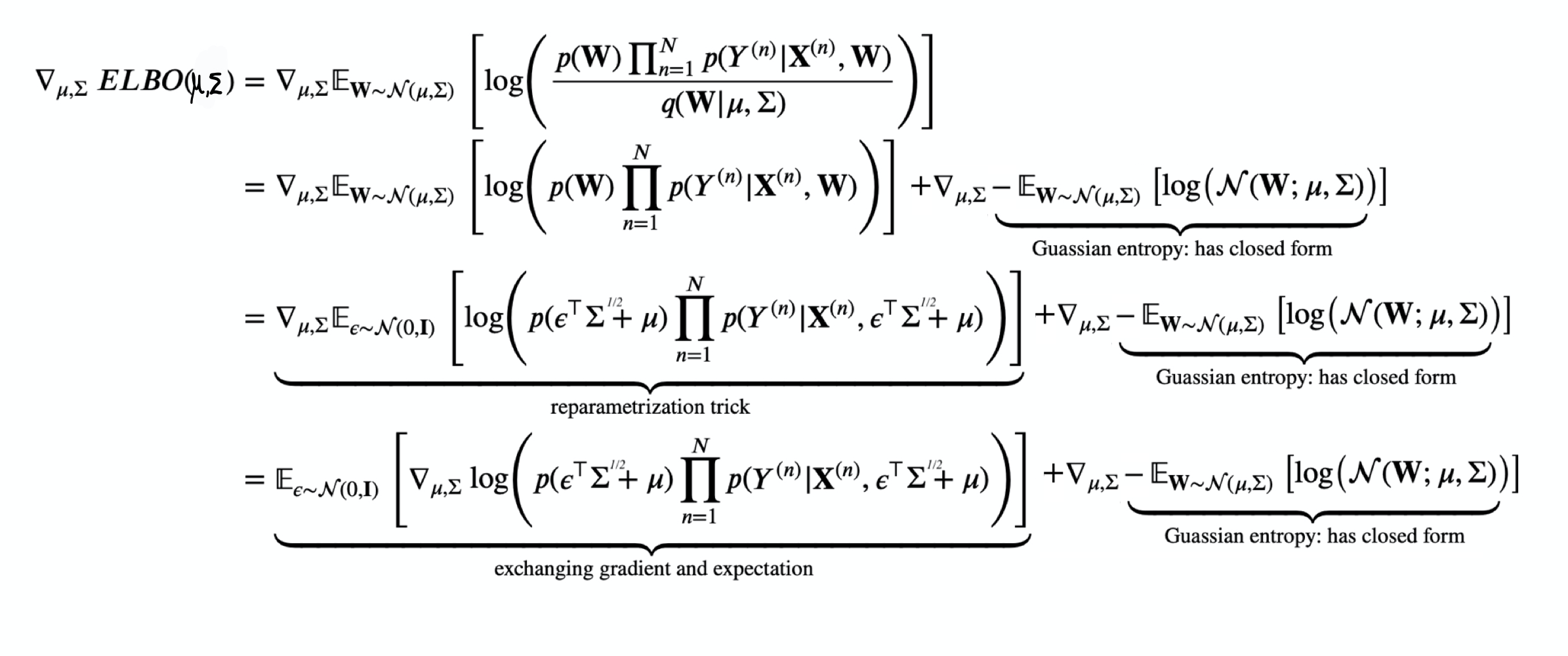
Black-Box Variational Inference with the Reparametrization Trick#
The Black-box Variational Inference (BBVI) with the reparametrization trick or Bayes By Backprop algorithm for BNN’s:
Initialization: pick an initial value \(\mu^{(0)}, \Sigma^{(0)}\)
Gradient Ascent: repeat:
Approximate the gradient
\[\begin{split}\begin{aligned} \nabla_{\mu, \Sigma} \, ELBO(\mu, \Sigma) \approx& \small\frac{1}{S} \sum_{s=1}^S \nabla_{\mu, \Sigma} \log \left[p(\epsilon_s^\top \Sigma^{1/2} + \mu) \prod_{n=1}^N p(Y^{(n)} | \mathbf{X}^{(n)}, \epsilon_s^\top \Sigma^{1/2} + \mu)\right] \\ &+ \nabla_{\mu, \Sigma}\underbrace{-\mathbb{E}_{\mathbf{W} \sim \mathcal{N}(\mu, \Sigma )}\left[\log \mathcal{N}(\mathbf{W};\mu, \Sigma ) \right]}_{\text{Guassian entropy: has closed form}}, \end{aligned}\end{split}\]where \(\epsilon_s \sim \mathcal{N}(0, \mathbf{I})\).
Update parameters \((\mu^{\text{current}}, \Sigma^{\text{current}}) \leftarrow (\mu^{\text{current}}, \Sigma^{\text{current}}) + \eta * {\text{reparametrization gradient}}\)
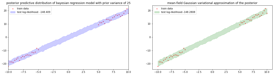
BBVI for Bayesian Linear Regression (Posterior Predictives)#
posterior_sample_size = 100
##visualize the posterior predictive of a bayesian polynomial regression model
#prior variance
prior_var = 5**2
fig, ax = plt.subplots(1, 2, figsize=(20, 5))
ax[0], joint_variance, joint_mean = bayesian_polynomial_regression(x_train, y_train, x_test, y_test, prior_var, y_var, ax[0], S=posterior_sample_size, poly_degree=1)
ax[1], var_variance, var_mean = variational_polynomial_regression(Sigma_W, sigma_y, x_test, y_test, x_train, y_train, forward, ax[1], posterior_sample_size=posterior_sample_size, S=4000, max_iteration=2000, step_size=1e-1, verbose=False)
plt.show()
Optimizing variational parameters...
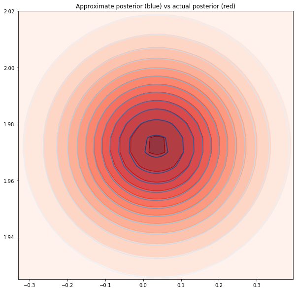
BBVI for Bayesian Linear Regression (Posteriors)#
#plot the target density against variational densities
fig, ax = plt.subplots(1, 1, figsize=(10, 10))
ax.contourf(x, y, z_p, levels=14, cmap='Reds', alpha=0.8)
ax.contour(x, y, z_p, levels=14, cmap='Reds', alpha=0.8)
ax.contour(x, y, z_q, levels=14, cmap='Blues', alpha=1.)
ax.set_title('Approximate posterior (blue) vs actual posterior (red)')
plt.show()
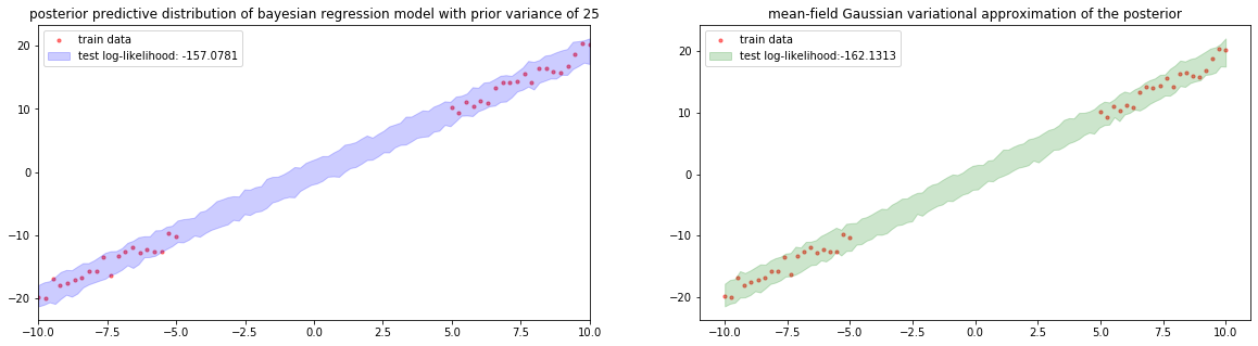
Optimizing variational parameters...
22.4. Summary#
(Width vs Depth) In a NN architecture, we control the width and the depth of the network. What is the effect of increasing each (independently) on the function that we learn?
|
|
|
Extremely wide NNs have fundamentally different behaviors than wide NNs
Reconciling modern machine learning practice and the bias-variance trade-off
Deep networks behave fundamentally differently than shallow but wide NNs
Exponential expressivity in deep neural networks through transient chaos
Deep networks can have unexpected pathologies
(Linear vs Neural Network Models) While both simple and complex models can be interpreted and successfully trained, there are trade-offs between using a complex vs a simple model!
Easily interpreted vs interpretations are harder to come by
Interpretations are more faithful vs interpretations can be more misleading
Training is easier (because objective function is convex) vs training is much harder (because objective function is extremely non-convex)
(Bayesian Neural Networks) Deep Bayes refers to the subfield of ML wherein we try to combine deep learning with Bayesian learning. A Bayesian Neural Network is one example of a deep Bayesian model.
Why do we want to make our NNs Bayesian?
How do we make NNs Bayesian?
How do we sample from the posterior?
Will sampling from the posterior using HMC going to work?
Can we do variational inference? Now we can - with 4 pieces of technology:
algebra tricks to get the gradient past the expectation in the ELBO
Monte Carlo estimate of the expectation in the ELBO
automatic differentiation
gradient descent
\[\begin{aligned} \nabla_{\mu, \Sigma}\,\underbrace{\mathbb{E}_{\mathbf{W} \sim q(\mathbf{W} | \mu, \Sigma)} \left[ \log \left( \frac{p(\mathbf{W}) \prod_{n=1}^N p(Y^{(n)} | \mathbf{X}^{(n)}, \mathbf{W})}{q(\mathbf{W} | \mu, \Sigma)} \right) \right]}_{ELBO(\mu, \Sigma)}. \end{aligned}\]
Variational Inference for BNNs#
The Black-box Variational Inference (BBVI) algorithm for BNN’s:
Initialization: pick an initial value \(\mu^{(0)}, \Sigma^{(0)}\)
Gradient Ascent: repeat:
Approximate the gradient
\[\begin{split}\begin{aligned} \nabla_{\mu, \Sigma} \, ELBO(\mu, \Sigma) &= \nabla_{\mu, \Sigma}\,\underbrace{\mathbb{E}_{\mathbf{W} \sim q(\mathbf{W} | \mu, \Sigma)} \left[ \log \left( \frac{p(\mathbf{W}) \prod_{n=1}^N p(Y^{(n)} | \mathbf{X}^{(n)}, \mathbf{W})}{q(\mathbf{W} | \mu, \Sigma)} \right) \right]}_{ELBO(\mu, \Sigma)}\\ &= \underbrace{\mathbb{E}_{\mathbf{W} \sim q(\mathbf{W} | \mu, \Sigma)}\left[ \nabla_{\mu, \Sigma}\, q(\mathbf{W} | \mu, \Sigma) * \log \left( \frac{p(\mathbf{W}) \prod_{n=1}^N p(Y^{(n)} | \mathbf{X}^{(n)}, \mathbf{W})}{q(\mathbf{W} | \mu, \Sigma)} \right) \right]}_{\text{score function gradient}}\\ &\approx\underbrace{\frac{1}{S}\sum_{s=1}^S \nabla_{\mu, \Sigma}\, \log q(\mathbf{W}^s | \mu, \Sigma) * \log \left( \frac{p(\mathbf{W}^s) \prod_{n=1}^N p(Y^{(n)} | \mathbf{X}^{(n)}, \mathbf{W}^s)}{q(\mathbf{W}^s | \mu, \Sigma)} \right)}_{{\text{MC approx. of score function gradient}}}, \end{aligned}\end{split}\]where \(\mathbf{W}^s\sim q(\mathbf{W} | \mu^{\text{current}}, \Sigma^{\text{current}})\).
Update parameters \((\mu^{\text{current}}, \Sigma^{\text{current}}) \leftarrow (\mu^{\text{current}}, \Sigma^{\text{current}}) + \eta * {\text{(MC approx. of score function gradient)}}\)
The reparametrization gradient is another way to push the gradient past the expectation in the gradient of the ELBO.
We note that since \(q(\mathbf{W} | \mu, \Sigma) = \mathcal{N}(\mathbf{W};\mu, \Sigma )\), sampling \(W\sim q(\mathbf{W} | \mu, \Sigma)\) is equivalent to sampling \(\epsilon \sim \mathcal{N}(0, \mathbf{I})\) and then transforming the sample \(\mathbf{W} = \epsilon^\top \Sigma^{1/2} + \mu\), where \(\mathbf{I}\) and \(\Sigma\) have the same dimensions.
Thus, we can rewrite the ELBO:
The Black-box Variational Inference (BBVI) with the reparametrization trick algorithm for BNN’s:
Initialization: pick an initial value \(\mu^{(0)}, \Sigma^{(0)}\)
Gradient Ascent: repeat:
Approximate the gradient
\[\begin{split}\begin{aligned} \nabla_{\mu, \Sigma} \, ELBO(\mu, \Sigma) \approx& \small\frac{1}{S} \sum_{s=1}^S \nabla_{\mu, \Sigma} \log \left[p(\epsilon_s^\top \Sigma^{1/2} + \mu) \prod_{n=1}^N p(Y^{(n)} | \mathbf{X}^{(n)}, \epsilon_s^\top \Sigma^{1/2} + \mu)\right] \\ &+ \nabla_{\mu, \Sigma}\underbrace{-\mathbb{E}_{\mathbf{W} \sim \mathcal{N}(\mu, \Sigma )}\left[\log \mathcal{N}(\mathbf{W};\mu, \Sigma ) \right]}_{\text{Guassian entropy: has closed form}}, \end{aligned}\end{split}\]where \(\epsilon_s \sim \mathcal{N}(0, \mathbf{I})\).
Update parameters \((\mu^{\text{current}}, \Sigma^{\text{current}}) \leftarrow (\mu^{\text{current}}, \Sigma^{\text{current}}) + \eta * {\text{reparametrization gradient}}\)
22.5. Exercises#
These problems were originally assigned as homework. Data files are in the book’s data/ folder. Worked solutions, where available, are collapsed beneath the questions they answer; try each problem before expanding them.
Problem Set: Bayesian Neural Networks#
Bayesian Neural Network Regression#
In this problem set you will explore Bayesian models for regression with neural networks – essentially, you will place priors on the network parameters \(\mathbf{W}\) and infer the posterior \(p(\mathbf{W}|\text{Data})\). These Bayesian models are called Bayesian neural networks. The data for this regression problem is in HW8_data.csv. You are provided an implementation of a neural network as well as an example of how to use it – but feel free to implement your own version!
Let’s instantiate a neural network with 1-hidden layer, 5-hidden nodes and relu activation:
Fit the neural network to the data and visualize the fit.
Exercise: Part I: Inference for Bayesian Neural Networks Using HMC
(The Bayesian Neural Network Model) We will implement the following Bayesian model for the data:
\[\begin{split}\begin{aligned} \mathbf{W} &\sim \mathcal{N}(0, 5^2 \mathbf{I}_{D\times D})\\ \mu^{(n)} &= g_{\mathbf{W}}(\mathbf{X}^{(n)})\\ Y^{(n)} &\sim \mathcal{N}(\mu^{(n)}, 0.5^2)\\ \end{aligned}\end{split}\]where \(g_{\mathbf{W}}\) is a neural network with parameters \(\mathbf{W}\) represented as a vector in \(\mathbb{R}^{D}\) with \(D\) being the total number of parameters (including biases).
Implement the log of the joint distribution inautograd’s version ofnumpy, i.e. implement \(\log \left[p(\mathbf{W})\prod_{n=1}^N p(Y^{(n)} |\mathbf{X}^{(n)} , \mathbf{W}) \right]\). Hint: you’ll need to write out the log of the various Gaussian pdf’s and implement their formulae usingautograd’s numpy functions.
Solution: Part I, Question 1
###Bayesian model parameterss
#covariance matrix of the Gaussian prior on weights
Sigma_W = 5**2 * np.eye(nn.D)
#Gaussian likelihood variance
sigma_y = 0.5**2
#number of data points
N = x_train.shape[1]
#precision matrix of the Gaussian prior on weights
Sigma_W_inv = np.linalg.inv(Sigma_W)
#determinant of the covaraince matrix of the Gaussian prior on weights
Sigma_W_det = np.linalg.det(Sigma_W)

###definition of the log prior
def log_prior(W):
    assert len(W.shape) == 2 and W.shape[1] == nn.D
    S = len(W)
    constant_W = -0.5 * (nn.D * np.log(2 * np.pi) + np.log(Sigma_W_det))
    exponential_W = -0.5 * np.diag(np.dot(np.dot(W, Sigma_W_inv), W.T))
    assert exponential_W.shape == (S, )
    log_p_W = constant_W + exponential_W
    return log_p_W

###definition of the log likelihood
def log_lklhd(W):
    assert len(W.shape) == 2 and W.shape[1] == nn.D
    S = W.shape[0]
    constant = (-0.5 * np.log(sigma_y) - 0.5 * np.log(2 * np.pi)) * N
    exponential = -0.5 * sigma_y**-1 * np.sum((y_train.reshape((1, 1, N)) - nn.forward(W, x_train))**2, axis=2).flatten()
    assert exponential.shape == (S, )
    return constant + exponential
(Sample from the Posterior) Use HMC to sample from the posterior of the Bayesian neural network in Question 1 with 1 hidden layer and 5 hidden nodes. Start with the following settings for your sampler:
params = {'step_size':1e-3,
          'leapfrog_steps':50,
          'total_samples':10000,
          'burn_in':.1,
          'thinning_factor':2,
          'position_init': nn.weights}
Note that you should initialize with the MLE model, otherwise convergence may be slow. Please feel free to tweak these design choices as you see fit!
Solution: Part I, Question 2
from autograd import numpy as np
from autograd import scipy as sp
from autograd import grad

class HMC:

    def __init__(self, potential_energy, kinetic_energy, kinetic_energy_distribution, random=None, diagnostic_mode=False):
        if random is not None:
            self.random = random
        else:
            self.random = np.random.RandomState(0)
        self.D = np.max(kinetic_energy_distribution(1).shape)
        self.potential_energy = potential_energy
        self.kinetic_energy = kinetic_energy
        self.total_energy = lambda position, momentum: potential_energy(position) + kinetic_energy(momentum)

        self.sample_momentum = lambda n: kinetic_energy_distribution(n).reshape((1, self.D))
        self.grad_potential_energy = grad(potential_energy)

        self.params = {'step_size': 0.1,
                       'leapfrog_steps': 10,
                       'total_samples': 1000,
                       'burn_in': 0.1,
                       'thinning_factor': 1,
                       'diagnostic_mode': diagnostic_mode}

        self.accepts = 0.
        self.iterations = 0.
        self.trace = np.empty((1, self.D))
        self.potential_energy_trace = np.empty((1,))

        assert self.sample_momentum(1).shape == (1, self.D)
        assert isinstance(self.potential_energy(self.sample_momentum(1)), float)
        assert isinstance(self.kinetic_energy(self.sample_momentum(1)), float)
        assert isinstance(self.total_energy(self.sample_momentum(1), self.sample_momentum(1)), float)
        assert self.grad_potential_energy(self.sample_momentum(1)).shape == (1, self.D)


    def leap_frog(self, position_init, momentum_init):
        # initialize position (a copy, so the caller's array is not changed in place)
        position = np.copy(position_init)

        # half step update of momentum
        momentum = momentum_init - self.params['step_size'] * self.grad_potential_energy(position_init) / 2

        # full leap frog steps
        for _ in range(self.params['leapfrog_steps'] - 1):
            position += self.params['step_size'] * momentum
            momentum -= self.params['step_size'] * self.grad_potential_energy(position)
            assert not np.any(np.isnan(position))
            assert not np.any(np.isnan(momentum))

        # full step update of position
        position_proposal = position + self.params['step_size'] * momentum
        # half step update of momentum
        momentum_proposal = momentum - self.params['step_size'] * self.grad_potential_energy(position_proposal) / 2


        return position_proposal, momentum_proposal

    def hmc(self, position_current, momentum_current):
        ### Refresh momentum
        momentum_current = self.sample_momentum(1)

        ### Simulate Hamiltonian dynamics using Leap Frog
        position_proposal, momentum_proposal = self.leap_frog(position_current, momentum_current)

        # compute total energy in current position and proposal position
        current_total_energy = self.total_energy(position_current, momentum_current)
        proposal_total_energy = self.total_energy(position_proposal, momentum_proposal)

        ### Output for diganostic mode
        if self.params['diagnostic_mode']:
            print('potential energy change:',
                  self.potential_energy(position_current),
                  self.potential_energy(position_proposal))
            print('kinetic energy change:',
                  self.kinetic_energy(momentum_current),
                  self.kinetic_energy(momentum_proposal))
            print('total enregy change:',
                  current_total_energy,
                  proposal_total_energy)
            print('\n\n')

        ### Metropolis Hastings Step
        # comute accept probability
        accept_prob = np.min([1, np.exp(current_total_energy - proposal_total_energy)])
        # accept proposal with accept probability
        if self.random.rand() < accept_prob:
            self.accepts += 1.
            position_current = np.copy(position_proposal)
            momentum_current = momentum_proposal

        return position_current, momentum_current

    def tuning(self, burn_in_period, position_init, momentum_init):
        ### Determine check point
        if self.params['diagnostic_mode']:
            check_point = 10
        else:
            check_point = 100

        ### Initialize position and momentum
        position_current = position_init
        momentum_current = momentum_init

        ### Tune step size param during burn-in period
        for i in range(burn_in_period):
            ### Checks accept rate at check point iterations and adjusts step size
            if i % check_point == 0 and i > 0:
                accept_rate = self.accepts / i
                print('HMC {}: accept rate of {} with step size {}'.format(i, accept_rate * 100., self.params['step_size']))

                if accept_rate < 0.5:
                    self.params['step_size'] *= 0.95
                if accept_rate > 0.8:
                    self.params['step_size'] *= 1.05

            ### perform one HMC step
            position_current, momentum_current = self.hmc(position_current, momentum_current)

        ### Reset number of accepts
        self.accepts = 0

        return position_current, momentum_current

    def run_hmc(self, check_point, position_init, momentum_init):
        ### Initialize position and momentum
        position_current = position_init
        momentum_current = momentum_init

        ### Perform multiple HMC steps
        for i in range(self.params['total_samples']):
            self.iterations += 1
            ### output accept rate at check point iterations
            if i % check_point == 0 and i > 0:
                accept_rate = self.accepts * 100. / i
                print('HMC {}: accept rate of {}'.format(i, accept_rate))

            position_current, momentum_current = self.hmc(position_current, momentum_current)

            # add sample to trace
            if i % self.params['thinning_factor'] == 0:
                self.trace = np.vstack((self.trace, position_current))
                self.potential_energy_trace = np.vstack((self.potential_energy_trace,
                                                         self.potential_energy(position_current)))

        self.trace = self.trace[1:]

    def sample(self, position_init=None, step_size=None, leapfrog_steps=None,
               total_samples=None, burn_in=None, thinning_factor=None, check_point=200,
               alpha=None, diagnostic_mode=None):

        ### Sample random initial momentum
        momentum_init = self.sample_momentum(1)

        ### Set model parameters
        if position_init is None:
            position_init = self.random.normal(0, 1, size=momentum_init.shape)
        else:
            assert position_init.shape == (1, self.D)
        if step_size is not None:
            self.params['step_size'] = step_size
        if leapfrog_steps is not None:
            self.params['leapfrog_steps'] = leapfrog_steps
        if total_samples is not None:
            self.params['total_samples'] = total_samples
        if burn_in is not None:
            self.params['burn_in'] = burn_in
        if thinning_factor is not None:
            self.params['thinning_factor'] = thinning_factor
        if diagnostic_mode is not None:
            self.params['diagnostic_mode'] = diagnostic_mode

        ### Tune parameters during burn-in period
        burn_in_period = int(self.params['burn_in'] * self.params['total_samples'])
        position_current, momentum_current = self.tuning(burn_in_period, position_init, momentum_init)
        ### Obtain samples from HMC using optimized parameters
        self.run_hmc(check_point, position_current, momentum_current)
        # (run_hmc already keeps every thinning_factor-th sample)
#potential energy function
def potential_energy(W):
    return -1 * (log_lklhd(W) + log_prior(W))[0]
#kinetic energy function
def kinetic_energy(W):
    return np.sum(W**2) / 2.0
#the gibbs distribution of the kinetic energy function
def kinetic_energy_distribution(n):
    return random.normal(0, 1, size=nn.D)
#initialize the position vector for HMC sampling with the weights of the trained neural network
position_init = nn.weights.reshape((1, nn.D))
#leap-frog step size
step_size = 1e-3
#leap-frog steps
leapfrog_steps = 50
#number of total samples after burn-in
total_samples = 10000
#percentage of samples to burn
burn_in = 0.1
#thinning factor
thinning_factor = 2

#instantiate an HMC sampler
HMC_sampler = HMC(potential_energy, kinetic_energy,
                  kinetic_energy_distribution,
                  random=random)

#sample from the bayesian neural network posterior
HMC_sampler.sample(position_init=position_init,
                   step_size=step_size,
                   leapfrog_steps=leapfrog_steps,
                   total_samples=total_samples,
                   burn_in=burn_in,
                   thinning_factor=thinning_factor)
HMC 100: accept rate of 100.0 with step size 0.001
HMC 200: accept rate of 100.0 with step size 0.0010500000000000002
HMC 300: accept rate of 100.0 with step size 0.0011025000000000002
HMC 400: accept rate of 100.0 with step size 0.0011576250000000002
HMC 500: accept rate of 100.0 with step size 0.0012155062500000004
HMC 600: accept rate of 100.0 with step size 0.0012762815625000006
HMC 700: accept rate of 100.0 with step size 0.0013400956406250007
HMC 800: accept rate of 100.0 with step size 0.0014071004226562508
HMC 900: accept rate of 99.8888888888889 with step size 0.0014774554437890634
HMC 200: accept rate of 99.5
HMC 400: accept rate of 99.25
HMC 600: accept rate of 99.0
HMC 800: accept rate of 98.875
HMC 1000: accept rate of 98.9
HMC 1200: accept rate of 99.0
HMC 1400: accept rate of 99.07142857142857
HMC 1600: accept rate of 99.1875
HMC 1800: accept rate of 99.27777777777777
HMC 2000: accept rate of 99.35
HMC 2200: accept rate of 99.4090909090909
HMC 2400: accept rate of 99.41666666666667
HMC 2600: accept rate of 99.46153846153847
HMC 2800: accept rate of 99.46428571428571
HMC 3000: accept rate of 99.43333333333334
[... 29 lines omitted ...]
HMC 9000: accept rate of 99.4
HMC 9200: accept rate of 99.40217391304348
HMC 9400: accept rate of 99.41489361702128
HMC 9600: accept rate of 99.41666666666667
HMC 9800: accept rate of 99.40816326530613
(Visualize the Posterior Predictive) Visualize 100 samples, randomly selected, from your posterior samples of \(\mathbf{W}\), by plotting their predicted values plus a random noise \(\epsilon \sim \mathcal{N}(0, 0.5^2)\) at 100 equally spaced x-values between -8 and 8:
x_test = np.linspace(-8, 8, 100)
y_test = nn.forward(sample, x_test.reshape((1, -1)))
y_test += np.random.normal(0, 0.5, size=y_test.shape)
where sample is a posterior sample of \(\mathbf{W}\).
Solution: Part I, Question 3
#100 randomly selected posterior samples
posterior_samples = HMC_sampler.trace[random.choice(len(HMC_sampler.trace), 100, replace=False)]
total_samples = len(posterior_samples)

y_predict_train_noiseless = nn.forward(posterior_samples, x_train).reshape((total_samples, -1))
y_pred_test = nn.forward(posterior_samples, x_test).reshape((total_samples, -1)) + np.random.normal(0, sigma_y**0.5, size=(total_samples, x_test.shape[1]))

#Gaussian log pdf
gaussian_log_pdf = lambda mu, sigma_sq, x: -0.5 * (np.log(2 * np.pi * sigma_sq) + (x - mu)**2 / sigma_sq)

#compute log likelihood for the training data
log_likelihood = []
for n in range(y_train.shape[1]):
    log_likelihood.append(gaussian_log_pdf(y_train[:, n], sigma_y,  y_predict_train_noiseless[:, n].flatten()).mean())
log_likelihood = np.array(log_likelihood).sum()

#compute the 95 percentiles and the mean of the posterior predictives
ub_bayes = np.percentile(y_pred_test, 97.5, axis=0)
lb_bayes = np.percentile(y_pred_test, 2.5, axis=0)
mean_bayes = np.mean(y_pred_test, axis=0)

#visualize the posterior predictive distribution
fig, ax = plt.subplots(1, 1, figsize=(10, 5))
for y_pred in y_pred_test:
    ax.plot(x_test.flatten(), y_pred, color='gray', alpha=0.1)
ax.scatter(x_train.flatten(), y_train.flatten(), color='red', s=10, alpha=0.5, label='train data')
ax.plot(x_test.flatten(), mean_bayes, '--', color='green', alpha=0.8, label='posterior mean')
ax.fill_between(x_test.flatten(), ub_bayes, lb_bayes, color='green', alpha=0.2, label='95% predictive interval')

ax.set_title('posterior predictive from HMC samples of the BNN posterior\n(train log-likelihood: {})'.format(np.round(log_likelihood, 4)))
ax.legend(loc='best')
plt.show()
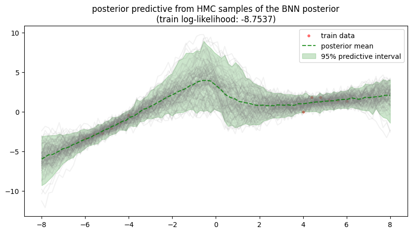
(Model Evaluation) Discuss the fit of your model to the data. Discuss also what the posterior predictive tell you about the aleatoric and epistemic uncertainty of the model. Are these uncertainties what you’d want (think about want kind of uncertainties you want and where)?
Exercise: Part II: Inference for BNNs Using Black-Box Variational Inference with the Reparametrization Trick
(BBVI with the Reparametrization Trick) Implement BBVI with the reparametrization trick for approximating an arbitrary posterior \(p(w| \text{Data})\) by an isotropic Gaussian \(\mathcal{N}(\mu, \Sigma)\), where \(\Sigma\) is a diagonal matrix. See the derivation earlier in this chapter or the example code from autograd’s github repo.
Unit Test: You should check that your implementation is correct by approximating the posterior of the following Bayesian logistic regression model:
\[\begin{split}\begin{aligned} w &\sim \mathcal{N}(0, 1)\\ Y^{(n)} &\sim Ber(\text{sigm}(wX^{(n)} + 10)) \end{aligned}\end{split}\]where \(w\), \(Y^{(n)}\), \(X^{(n)}\) are a real scalar valued random variables, and where the data consists of a single observation \((Y=1, X=-20)\).
The true posterior \(p(w | Y=1, X=-20)\) should look like the following (i.e. the true posterior is left-skewed):
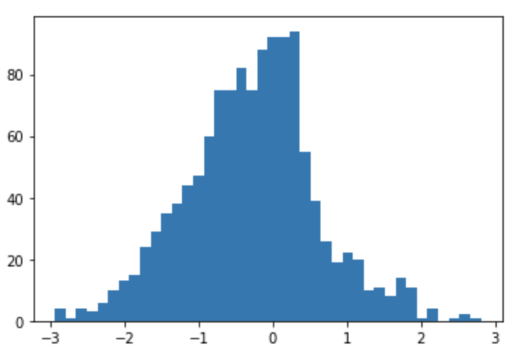
Your mean-field variational approximation should be a Gaussian with mean around -0.321 and standard deviation around 0.876.
Solution: Part II, Question 1
from autograd.misc.optimizers import adam, sgd
from autograd import numpy as np
from autograd import grad
from autograd.numpy import random as npr
import autograd.scipy.stats.multivariate_normal as mvn
import autograd.scipy.stats.norm as norm

import matplotlib.pyplot as plt


class BBVI:
    ''' BBVI with mean field approximation and reparameterization trick'''
    def __init__(self, log_probability, dimension, S=500, random=None, analytic_entropy=True, softplus=True):
        #instantiate random number generator
        if random is not None:
            self.random = random
        else:
            self.random = np.random.RandomState(0)
        self.D = dimension #dimension of support of target distribution
        self.S = S #number of monte carlo samples for computing expectation
        self.target = log_probability #target distribution
        self.unpack_params, self.variational_objective, self.gradient = self.make_variational_objective(analytic_entropy, softplus, log_probability)
        self.check_point = 100 #number of iterations before outputing optimization stats
        self.ELBO = np.empty((1, 1)) #elbo values over optimization
        self.variational_params = np.empty((1, 2 * self.D)) #variational parmeeters over optimization


    def make_variational_objective(self, analytic_entropy, softplus, log_probability):

        if softplus:
            def unpack_params(params):
                mean, parametrized_var = params[:self.D], params[self.D:]
                std = np.log(1 + np.exp(parametrized_var))
                return mean, std
        else:
            def unpack_params(params):
                mean, parametrized_var = params[:self.D], params[self.D:]
                std = np.exp(parametrized_var)
                return mean, std

        if analytic_entropy:
            def entropy(std):
                    ''' Gaussian entropy '''
                    return np.sum(0.5 * np.log(2 * np.pi * np.e) + np.log(std))

            def variational_objective(params, t):
                ''' Varational objective = H[q] + E_q[target] '''
                mean, std = unpack_params(params) #unpack std parameters
                samples = self.random.randn(self.S, self.D) * std + mean #sample from q using reparametrization
                lower_bound = entropy(std) +  np.mean(log_probability(samples, t)) #ELBO
                return -lower_bound
        else:
            def log_gaussian_pdf(samples, mean, std):
                assert samples.shape == (self.S, self.D)
                assert mean.shape == (1, self.D)

                Sigma = np.diag(std**2)
                Sigma_det = np.linalg.det(Sigma)
                Sigma_inv = np.linalg.inv(Sigma)

                constant = -0.5 * (self.D * np.log(2 * np.pi) + np.log(Sigma_det))
                dist_to_mean = samples - mean
                exponential = -0.5 * np.diag(np.dot(np.dot(dist_to_mean, Sigma_inv), dist_to_mean.T))
                return constant + exponential

            def variational_objective(params, t):
                mean, std = unpack_params(params) #unpack std parameters
                samples = self.random.randn(self.S, self.D) * std + mean #sample from q using reparametrization
                lower_bound = np.mean(log_probability(samples, t) - log_gaussian_pdf(samples, mean.reshape((1, self.D)), std)) #ELBO
                return -lower_bound

        return unpack_params, variational_objective, grad(variational_objective)

    def call_back(self, params, iteration, g):
        ''' Actions per optimization step '''
        elbo = -self.variational_objective(params, iteration)
        self.ELBO = np.vstack((self.ELBO, elbo))
        mean, std = self.unpack_params(params)
        self.variational_params = np.vstack((self.variational_params, np.hstack((mean, std)).reshape((1, -1))))
        if self.verbose and iteration % self.check_point == 0:
            print("Iteration {} lower bound {}; gradient mag: {}".format(iteration, elbo, np.linalg.norm(self.gradient(params, iteration))))

    def debug_call_back(self, params, iteration):
        ''' Actions per optimization step '''
        elbo = -self.variational_objective(params, iteration)
        self.ELBO = np.vstack((self.ELBO, elbo))
        self.variational_params = np.vstack((self.variational_params, params.reshape((1, -1))))
        if iteration % self.check_point == 0:
            print("Iteration {} lower bound {}; gradient mag: {}".format(iteration, elbo, np.linalg.norm(self.gradient(params, iteration))))

    def fit(self, step_size=1e-2, max_iteration=5000, check_point=None, params_init=None, call_back=None, verbose=True, optimizer='adam', mass=None, reset=True):
        ''' Optimization of the variational objective '''
        if check_point is not None:
            self.check_point = check_point

        if params_init is None:
            mean_init = self.random.normal(0, 0.1, size=self.D)
            parametrized_var_init = self.random.normal(0, 0.1, size=self.D)
            params_init = np.concatenate([mean_init, parametrized_var_init])

        assert len(params_init) == 2 * self.D

        self.verbose = verbose

        if call_back is None:
            call_back = self.call_back

        if reset:
            self.ELBO = np.empty((1, 1))
            self.variational_params = np.empty((1, 2 * self.D))

        if optimizer == 'adam':
            adam(self.gradient, params_init, step_size=step_size, num_iters=max_iteration, callback=call_back)
        elif optimizer == 'sgd':
            if mass is None:
                mass = 1e-16
            sgd(self.gradient, params_init, step_size=step_size, num_iters=max_iteration, callback=call_back, mass=mass)
        elif optimizer == 'debug':
            params = params_init
            for i in range(max_iteration):
                params -= step_size * self.gradient(params, i)
                self.debug_call_back(params, i)

        self.variational_params = self.variational_params[1:]
        self.ELBO = self.ELBO[1:]
Not covered here: a unit test of the implementation on the Bayesian logistic regression model.
(Variational Inference for BNNs) For the Bayesian model you implemented in Part I, Questions 1 and 2, use BBVI with the reparametrization trick to approximate the posterior of the Bayesian neural network with a mean-field Gaussian variational family (i.e. an isotropic Gaussian). Please set learning rate and maximum iteration choices as you see fit!
Solution: Part II, Question 2
#log joint distribution of the BNN (log_prior and log_lklhd are defined in Part I)
def log_joint(W, t):
    return log_lklhd(W) + log_prior(W)

#initialize the variational means at the MLE weights and the variational std's near zero
init_mean = nn.weights.reshape((nn.D, ))
init_var = np.ones(init_mean.shape) * -10
init = np.hstack((init_mean, init_var))

#fit a mean-field Gaussian approximation of the posterior with BBVI
#(with step size 1e-3 the ELBO is still rising after 10,000 iterations)
bbvi = BBVI(log_joint, nn.D, S=500, random=random)
bbvi.fit(step_size=1e-2, max_iteration=10000, check_point=1000, params_init=init)

#keep the variational parameters with the best ELBO over the last 100 iterations
best = np.argmax(bbvi.ELBO[-100:])
var_mean, var_std = np.split(bbvi.variational_params[-100:][best], 2)
Iteration 0 lower bound -185.87949140797616; gradient mag: 4.014578552818984
Iteration 1000 lower bound -63.77811252168141; gradient mag: 21.456917623534206
Iteration 2000 lower bound -56.43868191157114; gradient mag: 25.58634855369172
Iteration 3000 lower bound -52.841006026133215; gradient mag: 28.293362430983564
Iteration 4000 lower bound -52.41879774855775; gradient mag: 10.615756649916593
Iteration 5000 lower bound -53.46030481619978; gradient mag: 15.06745791428742
Iteration 6000 lower bound -48.59204013383875; gradient mag: 4.5042228032117
Iteration 7000 lower bound -48.95762556827522; gradient mag: 3.1676748578154115
Iteration 8000 lower bound -51.46443779733541; gradient mag: 3.071710774335043
Iteration 9000 lower bound -46.538403415330556; gradient mag: 18.246746703267746
(Visualize the Posterior Predictive) Visualize 100 samples \(\mathbf{W}^s\) from your approximate posterior of \(\mathbf{W}\) by plotting the neural network outputs with weight \(\mathbf{W}^s\) plus a random noise \(\epsilon \sim \mathcal{N}(0, 0.5^2)\) at 100 equally spaced x-values between -8 and 8:
x_test = np.linspace(-8, 8, 100)
y_test = nn.forward(sample, x_test.reshape((1, -1)))
y_test += np.random.normal(0, 0.5, size=y_test.shape)
where sample is a sample from the approximate posterior of \(\mathbf{W}\).
Solution: Part II, Question 3
#100 samples from the variational approximation of the posterior
posterior_samples = var_mean + var_std * random.randn(100, nn.D)
#posterior predictive samples: network outputs plus observation noise
y_pred_test = nn.forward(posterior_samples, x_test).reshape((100, -1)) + random.normal(0, sigma_y**0.5, size=(100, x_test.shape[1]))
#compute the 95% predictive interval and the predictive mean
y_postpred_ub = np.percentile(y_pred_test, 97.5, axis=0)
y_postpred_lb = np.percentile(y_pred_test, 2.5, axis=0)
y_postpred_means = np.mean(y_pred_test, axis=0)
#visualize 95% posterior predictive interval and posterior predictive mean
fig, ax = plt.subplots(1, 1, figsize=(10, 5))
for y_pred in y_pred_test:
    ax.plot(x_test.flatten(), y_pred, color='gray', alpha=0.1)
ax.scatter(x_train, y_train, color='red', label='training data')
ax.fill_between(x_test.flatten(), y_postpred_ub, y_postpred_lb,
                facecolor='blue', interpolate=True, alpha=0.1, label='posterior pred 95% interval')
ax.plot(x_test.flatten(), y_postpred_means, color='blue', linestyle='--', linewidth=1, label='posterior pred mean')
ax.legend(loc='best')
plt.show()
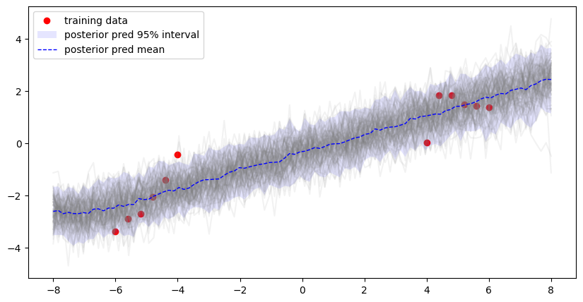
(Model Evaluation) Discuss the fit of your model to the data. Discuss also what the posterior predictive tell you about the aleatoric and epistemic uncertainty of the model. Are these uncertainties what you’d want (think about want kind of uncertainties you want and where)?
Exercise: Part III: Comparison
(Model Evaluation) Compare the posterior predictive visualization from BBVI with the reparametrization trick to the one you obtained using HMC. Can you say whether or not your posterior approximation is good? How does approximating the posterior effect our estimation of epistemic and aleatoric uncertainty?
Solution: Part III, Question 1
Compare the posterior predictive in Part II, Question 3 with the one produced by HMC in Part I, Question 3.
In general, it looks like the posterior predictive uncertainty produced by variational inference is smaller across the x-values we tested. In addition, the posterior predictive produced by HMC was able to capture epistemic uncertainty – the predictive uncertainty where there is no training data is larger than where there is training data; whereas the predictive uncertainty produced by variational inference is rather uniform across the input space regardless of whether or not training data is present.
Not covered here: whether the posterior approximation is good.
(Quality of Posterior Vs Quality of Posterior Predictive) Based on your convergence diagnostics of your HMC sampler, do you believe that you’ve obtained a set of representative samples from the BNN posterior? Why or why not?
Based on your understanding of BNN posteriors, do you believe that a mean-field Gaussian is a good approximation of the BNN posterior? Why or why not?
Which set of samples, HMC or VI, do you believe better captures the BNN posterior?
Based on the empirical results from above, do you believe there is a clear positive relationship between posterior approximation and quality of posterior predictive uncertainties - i.e. is it true that the more I capture of the BNN posterior the better the quality of my posterior predictive uncertainties?
Solution: Part III, Question 2
#visualize the traceplots for all of the 16 neural network parameters
fig, ax = plt.subplots(4, 4, figsize=(20, 20))
for i in range(nn.D):
    row = i // 4
    col = i % 4
    ax[row, col].plot(range(len(HMC_sampler.trace)), HMC_sampler.trace[:, i], color='gray', alpha=0.7)
fig.suptitle('Trace plots for all neural network parameters', y=0.9)
plt.show()
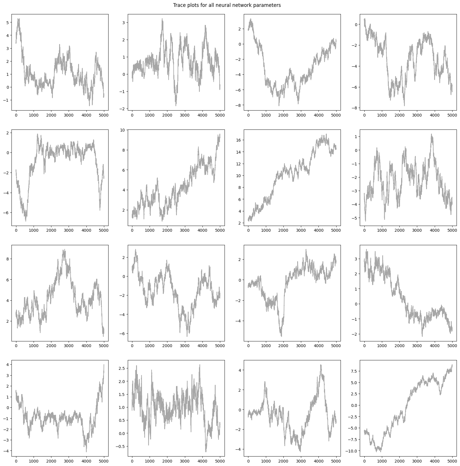
As we can see, none of the parameters have converged.
Not covered here: whether a mean-field Gaussian is a good approximation of the BNN posterior, which set of samples better captures it, and how posterior approximation relates to the quality of the posterior predictive uncertainties.
(Speed and Scalability) Compare the two inference methods, HMC and BBVI, and discuss the scalability of each with respect to the number of model parameters and number of data points (how does increasing the number of model parameters or the number of data points affect each inference method?).
22.6. Further Reading#
Variational Inference for Bayesian Neural Networks