Logistic Regression and Gradient Descent

15. Logistic Regression and Gradient Descent#

This chapter is adapted from AM207 (Harvard, Fall 2021). Watch the recorded lecture.

In this chapter

Logistic Regression
Gradient Descent
Convex Optimization

15.1. Logistic Regression#

Coin-Toss Revisited: Modeling a Bernoulli Variable with Covariates#

Let’s revisit our model for coin-toss: we’d assumed that the outcomes $Y^{(n)}$ were independently and identically distributed as Bernoulli’s, $Y^{(n)} \sim Ber(\theta)$. In this chapter, we will re-examine the identical part of the modeling assumptions.

Realistically, the probability of $Y^{(n)} = 1$ depends on variables like force, angle, spin etc.

Let $\mathbf{X}^{(n)} \in \mathbb{R}^D$ be $D$ number of such measurements of the $n$-th toss. We model the probability of $Y^{(n)} = 1$ as a function of these covariates $\mathbf{X}^{(n)}$:

\[ Y^{(n)} \sim Ber\left(\mathrm{sigm}\left(f\left(\mathbf{X}^{(n)}; \mathbf{w}\right)\right)\right) \]

where $\mathbf{w}$ are the parameters of $f$ and $\mathrm{sigm}$ is the sigmoid function $\mathrm{sigm}(z) = \frac{1}{1 + e^{-z}}$.

Note: we need the sigmoid function to transform an arbitrary real number $f\left(\mathbf{X}^{(n)}; \mathbf{w}\right)$ into a probability (i.e. a number in $[0, 1]$).

The Logistic Regression Model#

Given a set of $N$ observations $(\mathbf{x}^{(1)}, y^{(1)}), \ldots, (\mathbf{x}^{(N)}, y^{(N)})$. We assume the following model for the data.

\[ Y^{(n)} \sim Ber\left(\mathrm{sigm}\left(f\left(\mathbf{X}^{(n)}; \mathbf{w}\right)\right)\right). \]

This is called the logistic regression model.

Fitting this model on the data means inferring the parameters $\mathbf{w}$ that best aligns with the observations.

Once we have inferred the parameters $\mathbf{w}$, given a new set of covariates $\mathbf{x}^{\text{new}}$, we can predict the probability of $\mathbf{Y}^{\text{new}} = 1$ by computing

\[\mathrm{sigm}\left(f\left(\mathbf{X}^{(n)}; \mathbf{w}\right)\right).\]

For now, we will assume that $f$ is a linear function:

\[ f\left(\mathbf{X}^{(n)}; \mathbf{w}\right) = \mathbf{w}^\top \mathbf{X}^{(n)}. \]

Going deeper: The Relationship Between Logistic Regression and Classification

What Is Classification? A regression problem is where we predict a quantitative outcome $y$ based on some covariates $x$.

Example: Given the number of room, the number of allowed guests and the neighborhood, predict price of an Airbnb listing.

A classification problem is a categorical outcome $y$ based on some covariates $x$.

Example: Given the age, education and income level of a loan applicant, predict whether or not the loan application will be approved.

How Do We Classify? The data for classification consists of a set of tuples $(\mathbf{x}^{(n)}, y^{(n)})$, where $\mathbf{x}^{(n)}\in \mathbb{R}^D$ is a set of predictors/covariates (e.g. age, income etc) for the $n$-th observation and $y^{(n)}$ is the binary label (e.g. did the person receive the loan). The set of observations that are labeled $y=0$ are called class 0 and the set labeled $y=1$ are called class 1.

The goal is learn a function $f(\mathbf{x})$ so that given a new set of covariates $\mathbf{x}$ we can predict the corresponding label $y$.

Suppose our data has a small number of predictors, by visualizing the data we can intuitively check how easy it is to separate the classes. In the following example, we have two covariates. We scatter plot the covariates (pictured as crosses and bars), we then indicate data belonging to class 1 by visualizing them as blue crosses and those belonging to class 0 as red bars.

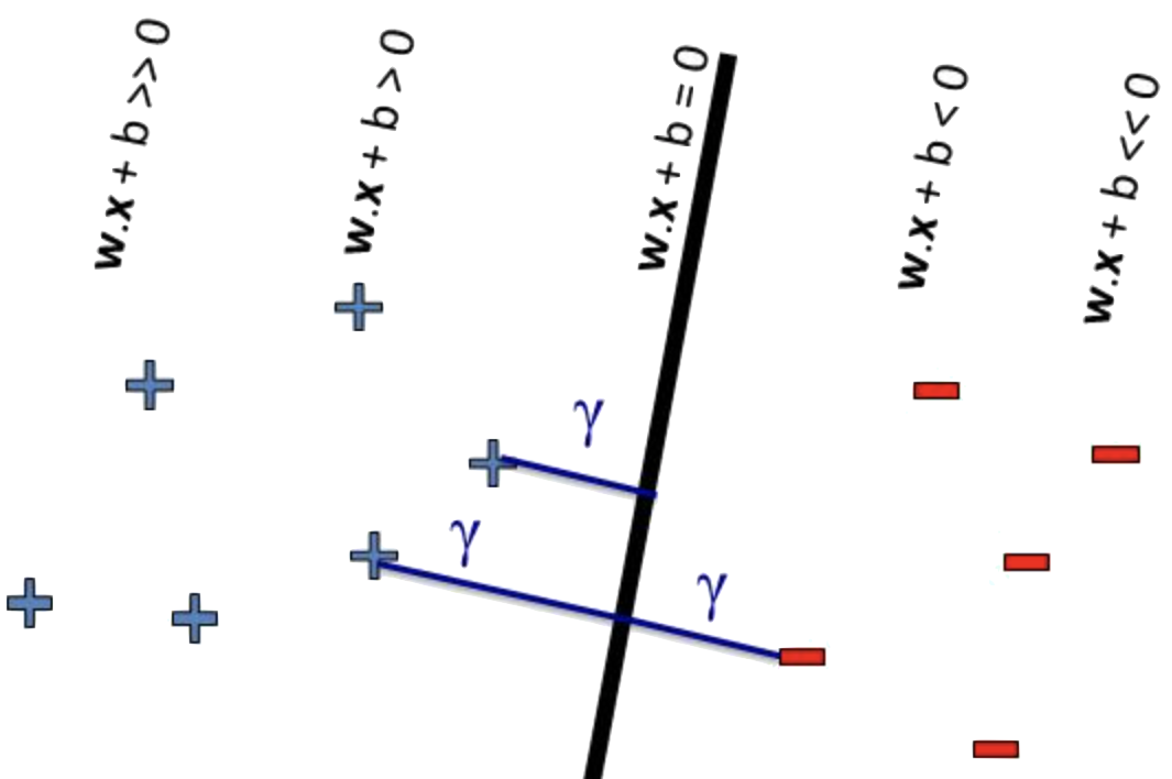
Ideally, the classes are easily separated by a curve (or surface) in the input space, this curve (or surface) is called the decision boundary.

When the decision boundary is linear (i.e. a line or a plane), it is defined by the equation

\[ \mathbf{w}^\top \mathbf{x} = w_0x_0 + w_1x_1 + \ldots + w_D x_D = 0 \]

where $x_0 = 1$. Often we write $b = w_0x_0$ and we call $b$ the bias term.

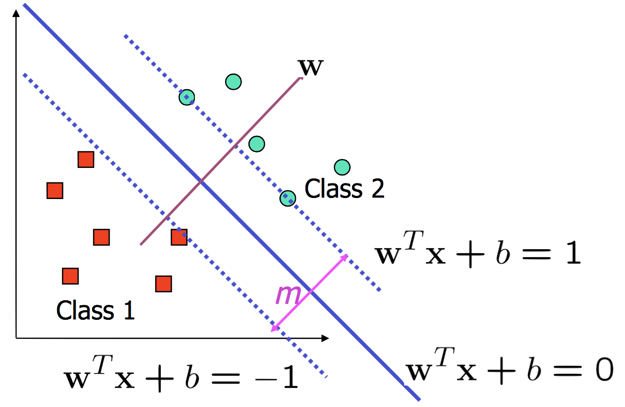
The vector $\mathbf{w}$ allow us to gauge the ‘distance’ of a point from the decision boundary. That is, the magnitude of the inner product $|\mathbf{w}^\top \mathbf{x}|$ gives us the distance between the point $\mathbf{x}$ and the decision boundary, whereas the sign of $\mathbf{w}^\top \mathbf{x}$ gives us the side of the decision boundary on which the point $\mathbf{x}$ lies. The proof of this is short and geometric – you should try to work it out!

(In the picture below, they use $\mathbf{w}^\top \mathbf{x}$ to express $w_1x_1 + \ldots + w_D x_D + b$, whereas we pretend that $x_0 = 1$ and $b = w_0x_0$. This is just a difference in notation)

Once we have a decision boundary should we always classify points on one side of the boundary as 1 and points on the other side as 0?

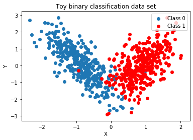
For classes that are not linearly separable (the classes don’t fall cleanly along two sides of a linear decision boundary), we want to make “soft classifications”. That is, rather than declaring $y=1$ when $\mathbf{w}^\top \mathbf{x} > 0$ and $y=0$ when $\mathbf{w}^\top \mathbf{x} <0$, we want to encode uncertainty in our prediction of the label $y$. We want to say the following:

When $\mathbf{x}$ is very far from the decision boundary, i.e. when $|\mathbf{w}^\top \mathbf{x}|$ is very large, and when $\mathbf{w}^\top \mathbf{x}>0$ then we want to say $y=1$ with high probability (analogously, when $\mathbf{x}$ is very far from the decision boundary and $\mathbf{w}^\top \mathbf{x}<0$, we want to say $y=0$ with high probability). When $\mathbf{x}$ is very close from the decision boundary, i.e. when $|\mathbf{w}^\top \mathbf{x}|\approx 0$, we want to be maximally uncertain about how predict $y$, i.e. we predict $y$ randomly by a 50-50 chance.

Formalizing this: to model the probability of labeling a point a certain class, we have to convert distance, $\mathbf{w}^\top\mathbf{x}$ (which is unbounded) into a number (probability) between 0 and 1, using the sigmoid function:

\[ \text{Prob}(y = 1 | \mathbf{x}) = \text{sigm}(\underbrace{\mathbf{w}^\top\mathbf{x}}_{\text{distance}}) \]

where $\text{sigm}(z) = \frac{1}{1 + e^{-z}}$. This way, when $\mathbf{w}^\top\mathbf{x}$ is large and positive then $\text{sigm}(\underbrace{\mathbf{w}^\top\mathbf{x}}_{\text{distance}})$ is close to 1, when $\mathbf{w}^\top\mathbf{x}$ is large and negative then $\text{sigm}(\underbrace{\mathbf{w}^\top\mathbf{x}}_{\text{distance}})$ is close to 0; when $\mathbf{w}^\top\mathbf{x}$ is near 0 then $\text{sigm}(\underbrace{\mathbf{w}^\top\mathbf{x}}_{\text{distance}})$ is close to 0.5, i.e. $\text{Prob}(y = 1 | \mathbf{x}) = 0.5$. This is exactly what we wanted!

Interpreting a Logistic Regression Model#

Suppose that you fit a logistic regression model to predict whether a loan application should be approved. Suppose that you have three covariates:

x_1 representing gender: 0 for male, 1 for female
x_2 for the income
x_3 for the loan amount

Suppose that the parameters you found are:

\[ p(y=1 | x_1, x_2, x_3) = \mathrm{sigm}(-1 + 3 x_1 + 1.5 x_2 + 1.75 x_3). \]

What are the parameters telling us about the most influential attribute for predicting loan approval? What does this say about our data?

With Great Explanatory Power Comes Great Responsibility!#

So in the previous predictive model for loan application model we’d use the following covariates:

x_1 representing gender: 0 for male, 1 for female
x_2 for the income
x_3 for the loan amount

We were pleased that using covariates we can hypothesize why the outcome $y$ is a certain way - why is the loan approved or denied. But just because we can collect the data for the covariates does it mean that we should use them? It particular, in our logistic model above, the most impactful factor on a loan decision was gender, does this seem reasonable? Should we use this model in real-life loan decisions?

In models that are built on human data, covariates containing information that infringes on the rights of the subject to remain anonymous or to keep potentially non-relevant and biasing information out of the decision making process are called sensitive or protected attributes.

When not to use sensitive/protected attributes#

Gender, in the case of loan decisions, is a protected attribute, since under the Equal Credit Opportunity Act makes it illegal for a creditor to discriminate in any aspect of credit transaction based on certain characteristics including gender. Thus, any decision process using gender to inform a loan decision can be potentially considered discriminatory.

In fact, most credit models used in industry are trained on data that are stripped of protected attributes - meaning that these models never see covariates like gender during training or deployment!

If we had deployed the logistic model to make real life loan decisions, not only would our decisions be potentially unfair and possibly questionable in terms of financial soundness (since our decisions are heavily influenced by a covariate not directly related to the financial qualifications of a loan applicant), using such a model exposes our company to regulatory sanctions and law-suits.

When you might want to use sensitive/protected attributes#

So should we never collect data on protected attributes? Well, unfortunately, just because we are blind to protected attributes it does not mean that our decisions are fair with respect to these attributes! That is, just because we don’t see gender when making decisions, it does not mean that our decisions impact men and women equally. In fact, the Equal Credit Opportunity Act contains explicit language that protects consumers from the disparate impact of credit decision systems. Disparate impact is defined as the unequal impact of a credit policy on a legally protected class:

“A lender’s policies, even when applied equally to all its credit applicants, may have a negative effect on certain applicants. For example, a lender may have a policy of not making single family home loans for less than $60,000. This policy might exclude a high number of applicants who have lower income levels or lower home values than the rest of the applicant pool. That uneven effect of the policy is called disparate impact.”

How do modelers and engineers prevent their models from creating disparate impact for protected classes of people? One of the key ways to check for disparate impact is to compare model decisions on protected classes against model decisions against the population (for example, we can compare the percentages of loans the model approves for men and for women). But in order perform these checks, we need access to protected attributes!

Often times, the models we are auditing for disparate impact are “black-boxes”, that is, the inner workings of the model (as well as details like the training procedure) are all proprietary information and we only have access to the models inputs and outputs, $(x_2, x_3, y)$ (note that the black-box model is not using the protected attribute gender $x_1$). In these cases, we can train a proxy model on covariates including protected attributes as well as the predictions of the black-box model, and then analyze our proxy model as an approximation to the black-box model. If we suppose that our logistic regression model above was a proxy model that is trained to approximate a black-box model, then our proxy model is telling us that the black-box model’s decisions are highly correlated with gender and hence it’s decisions may cause disparate impact! This is a case where we needed to look at protected attributes in order to check for regulatory compliance!

So why is this happening - why is a black-box model that is trained on data stripped of gender information making decisions that are highly correlated with gender? There are many possible explanations for this, but one common reason for this is that gender is a confounding variable, that is, some combination of income and loan amount is secretly encoding for gender (e.g. let’s say that in your data set, all the men earn 50k-60k and apply for exactly $10,000 of loans) and the black-box model is implicitly relying on gender to make loan decisions.

Appropriate usage of sensitive/protected attributes#

So now we see that protected attributes can be extremely useful when we are auditing models for regulatory compliance, should we collect sensitive or protected attributes all the time and as many of them as possible? Unfortunately, it’s not so simple: some industries are required by law to collect sensitive attribute data, while others are prohibited from doing so, still others infer sensitive attributes from collected data for compliance checking purposes (e.g. using income and other covariates to infer gender or zip codes to infer race). While useful for antidiscriminatory purposes, collecting or inferring sensitive protected attribute is nonetheless full of challenges and potential pitfalls (for example, protected attributes you inferred can violate the subject’s right to non-disclosure!) - references in this section addresses the issues of appropriate usage of sensitive attributes.

Furthermore, how you collect and encode ata can deeply impact your fairness/compliance analysis. For example, application forms that include two options for gender and three boxes for race may cause us to incorrectly aggregate subjects who do not fall neatly into these boxes under categories that are inappropriate (and by the way, we’ve not been carefully distinguishing gender and sex in this discussion, but they maybe treated differently under different bodies of laws. Also, are they equivalent concepts to our human subjects from whom we are collecting the data? What are we really trying to measure by collecting gender or sex data?). Such misleading categorization can cause us to miss cases of disparate impact in our analysis, since we have simply missed out on important subgroups of the population.

If you feel like we’re now treading in the unfamiliar territories of social science or law, you are not mistaken! When we work with human data, the interpretation of the data and hence our analysis hinges on our ability to meaningfully understand the data in social contexts and in human terms. Just as we need to consult physicist domain experts when we are building a statistical model for physical data, medical experts when we are building models for medical data, when we build models that have social impact we have to proceed carefully under the advisement of experts on our social/legal systems.

References for Issues Involving Proper Use of Protected Attributes

Going deeper: Interpreting a Logistic Regression Model: Log-Odds

A more formal way of interpreting the parameters of the logistic regression model is through the log-odds. That is, we solve for $\mathbf{w}^\top\mathbf{x}$ in terms of $\text{Prob}(y = 1 | \mathbf{x})$.

\[\begin{split}\begin{aligned} \text{Prob}(y = 1 | \mathbf{x}) &= \text{sigm}(\mathbf{w}^\top\mathbf{x})\\ \text{sigm}^{-1}(\text{Prob}(y = 1 | \mathbf{x})) &= \mathbf{w}^\top\mathbf{x}\\ \log \left( \frac{\text{Prob}(y = 1 | \mathbf{x})}{1 - \text{Prob}(y = 1 | \mathbf{x})}\right)&= \mathbf{w}^\top\mathbf{x}\\ \log \left( \frac{\text{Prob}(y = 1 | \mathbf{x})}{\text{Prob}(y = 0 | \mathbf{x})}\right)&= \mathbf{w}^\top\mathbf{x} \end{aligned}\end{split}\]

where we used the fact that $\text{sigm}^{-1}(z) = \frac{z}{1 - z}$.

The term $\log \left( \frac{\text{Prob}(y = 1 | \mathbf{x})}{\text{Prob}(y = 0 | \mathbf{x})}\right)$ is essentially a ratio of the probability of $y=1$ and the probability of $y=0$, we can interpret this quantity as the (log) odds of you winning if you’d bet that $y=1$. Thus, we can imagine the parameter $w_d$ for the covariate $x_d$ as telling us if the odd of winning a bet on $y=1$ is good.

if $w_d < 0$, then by increasing $x_d$ (while holding all other covariates constant) we make $\mathbf{w}^\top\mathbf{x}$ more negative, and hence the ratio $\frac{\text{Prob}(y = 1 | \mathbf{x})}{\text{Prob}(y = 0 | \mathbf{x})}$ closer to 0. That is, when $w_d < 0$, increasing $x_d$ decreases our odds.
if $w_d > 0$, then by increasing $x_d$ (while holding all other covariates constant) we make $\mathbf{w}^\top\mathbf{x}$ more positive, and hence the ratio $\frac{\text{Prob}(y = 1 | \mathbf{x})}{\text{Prob}(y = 0 | \mathbf{x})}$ larger. That is, when $w_d > 0$, increasing $x_d$ decreases our odds.

Maximizing the Logistic Regression Log-likelihood#

Given a set of $N$ observations $(\mathbf{x}^{(1)}, y^{(1)}), \ldots, (\mathbf{x}^{(N)}, y^{(N)})$. We want to find $\mathbf{w}_{\text{MLE}}$ that maximizes the log (joint) likelihood:

\[\begin{split}\begin{aligned} \small \mathbf{w}_{\text{MLE}} =& \underset{\mathbf{w}}{\mathrm{argmax}}\;\ell(\mathbf{w}) \equiv \underset{\mathbf{w}}{\mathrm{argmin}}\;-\ell(\mathbf{w}) =\underset{\mathbf{w}}{\mathrm{argmin}}-\log \prod_{n=1}^N p(y^{(n)} | \mathbf{x}^{(n)}) \\ =& \underset{\mathbf{w}}{\mathrm{argmin}}\sum_{n=1}^N -\log\left( \mathrm{sigm}(\mathbf{w}^\top \mathbf{x}^{(n)})^{y^{(n)}}(1 -\mathrm{sigm}(\mathbf{w}^\top \mathbf{x}^{(n)}))^{1 - y^{(n)}} \right) \\ =& \underset{\mathbf{w}}{\mathrm{argmin}}\sum_{n=1}^N -y^{(n)}\,\log\,\mathrm{sigm}(\mathbf{w}^\top \mathbf{x}^{(n)}) \\ &- (1 - y^{(n)}) \log (1 -\mathrm{sigm}(\mathbf{w}^\top \mathbf{x}^{(n)})) \end{aligned}\end{split}\]

Optimizing the likelihood requires us to find the stationary points of the gradient of $\ell(\mathbf{w})$:

\[ \nabla_{\mathbf{w}} \ell(\mathbf{w}) = -\sum_{n=1}^N \left(y^{(n)} - \frac{1}{1 + e^{-\mathbf{w}^\top\mathbf{x}^{(n)}}} \right) \mathbf{x}^{(n)} =\mathbf{0} \]

Can we solve for $\mathbf{w}$?

15.2. Gradient Descent#

Gradient as Directional Information#

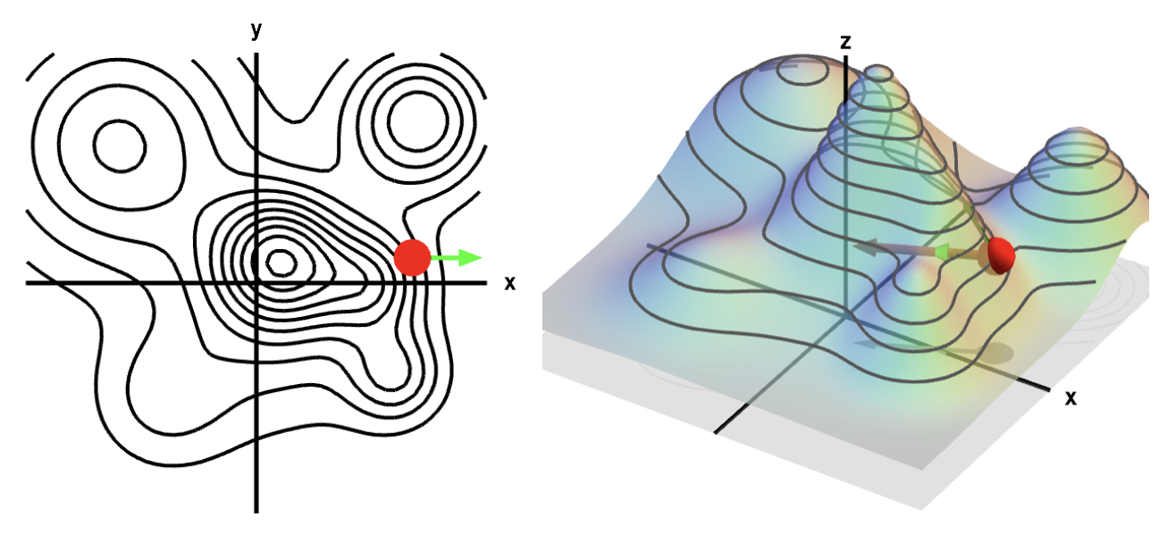
The gradient is orthogonal to the level curve of $f$ at $x^*$ and hence, when it is not zero, points in the direction of the greatest instantaneous increase in $f$.

An Intuition for Gradient Descent#

The intuition behind various flavours of gradient descent is as follows:

Download the derivation (PDF)

Gradient Descent: the Algorithm#

start at random place: $\mathbf{w}^{(0)}\leftarrow \textbf{random}$
until (stopping condition satisfied):

a. compute gradient at $\mathbf{w}^{(t)}$: gradient ($\mathbf{w}^{(t)}$) = $\nabla_{\mathbf{w}}$ loss_function ($\mathbf{w}^{(t)}$)

b. take a step in the negative gradient direction: $\mathbf{w}^{(t+1)} \leftarrow \mathbf{w}^{(t)}$ - $\eta$ * gradient ($\mathbf{w}^{(t)}$)

Here $\eta$ is called the learning rate.

Diagnosing Design Choices with the Trajectory#

If this is your objective function during training, what can you conclude about your step-size?

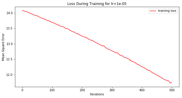
Diagnosing Issues with the Trajectory#

If this is your objective function during training, what can you conclude about your step-size?

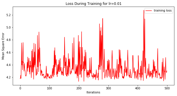
If this is your objective function during training, what can you conclude about your step-size?

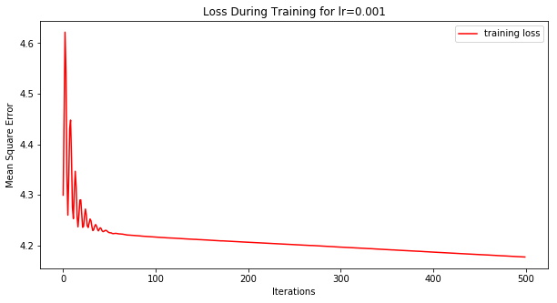
Gradient Descent: Step Size Matters#

Gradient Descent for Logistic Regression#

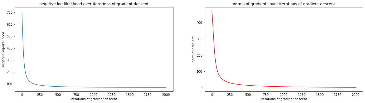
When diagnosing our gradient descent learning, we can:

Visualize the log-likelihood. What does this tell us?
Visualize the norm of the gradients. What does this tell us?

What else should we visualize to check that our learned model aligns with the data?

Show code cell content

Hide code cell content

# generate 2d classification dataset
centers = [[1, 1], [-1, -1]]
X, y = make_blobs(n_samples=400, n_features=2, centers=centers)
X = np.hstack((X, np.ones((X.shape[0], 1))))

#define the sigmoid function
sigmoid = lambda z: 1. / (1. + np.exp(-z))

#define the negative log-likelihood
nll = lambda X, y, w:  -(y * np.log(sigmoid(X.dot(w))) + (1 - y) * np.log(1 - sigmoid(X.dot(w)))).sum()

#define logistic regression MLE inference by gradient descent
def logistic_regression_fit(X, y, init=None, threshold=1e-6, total_iterations=1000, eta=1e-4):
    #implement the gradient
    gradient = lambda w: -((y - sigmoid(X.dot(w)))[:, np.newaxis] * X).sum(axis=0)
    
    #initialize parameters w
    if init is None:
        init = np.random.normal(0, 1, size=X.shape[1])
    w_current = init
    #store the negative log-likelihood
    nlls = []
    #store the norm of the gradients 
    grad_norms = []
    #initialize the difference between current and new parameters
    delta = 1
    i = 0
    #gradient descent 
    while i < total_iterations and delta > threshold:
        #compute the gradient
        grad = gradient(w_current)
        #update parameter by taking gradient step
        w_next = w_current - eta * grad
        #compute the difference between current parameters and new parameters
        delta = np.linalg.norm(w_next - w_current)
        #compute the norm of the gradient
        grad_norms.append(np.linalg.norm(grad))
        #compute the negative log-likelihood
        nlls.append(nll(X, y, w_current))
        
        w_current = w_next
        i += 1
        
    return w_current, nlls, grad_norms

def plot_diagnostics(ax, nlls, grad_norms):
    ax[0].plot(range(len(nlls)), nlls)
    ax[0].set_title('negative log-likelihood over iterations of gradient descent')
    ax[0].set_ylabel('negative log-likelihood')
    ax[0].set_xlabel('iterations of gradient descent')

    ax[1].plot(range(len(grad_norms)), grad_norms, color='red')
    ax[1].set_title('norms of gradients over iterations of gradient descent')
    ax[1].set_ylabel('norm of gradient')
    ax[1].set_xlabel('iterations of gradient descent')
    return ax

w_MLE, nlls, grad_norms = logistic_regression_fit(X, y, init=None, threshold=1e-6, total_iterations=2000, eta=1e-4)

fig, ax = plt.subplots(1, 2, figsize=(20, 5))
ax = plot_diagnostics(ax, nlls, grad_norms)
plt.show()

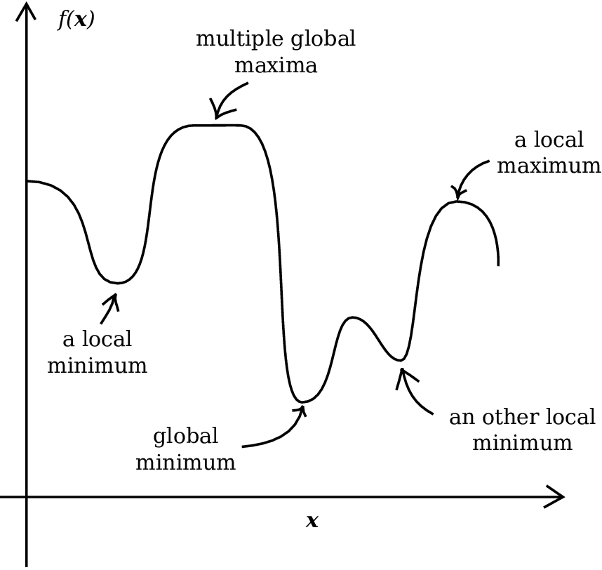
../_images/a75b6c54a7cd03fe9c2637c28f89810f5353c9b572d42d16c0093a09ed48390d.png

But Did We Optimize It?#

15.3. Convex Optimization#

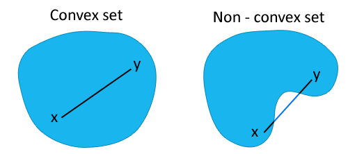
Convex Sets#

A convex set $S\subset \mathbb{R}^D$ is a set that contains the line segment between any two points in $S$. Formally, if $x, y \in S$ then $S$ contains all convex combinations of $x$ and $y$:

\[ tx + (1-t) y \in S,\quad t\in [0, 1]. \]

Convex Functions#

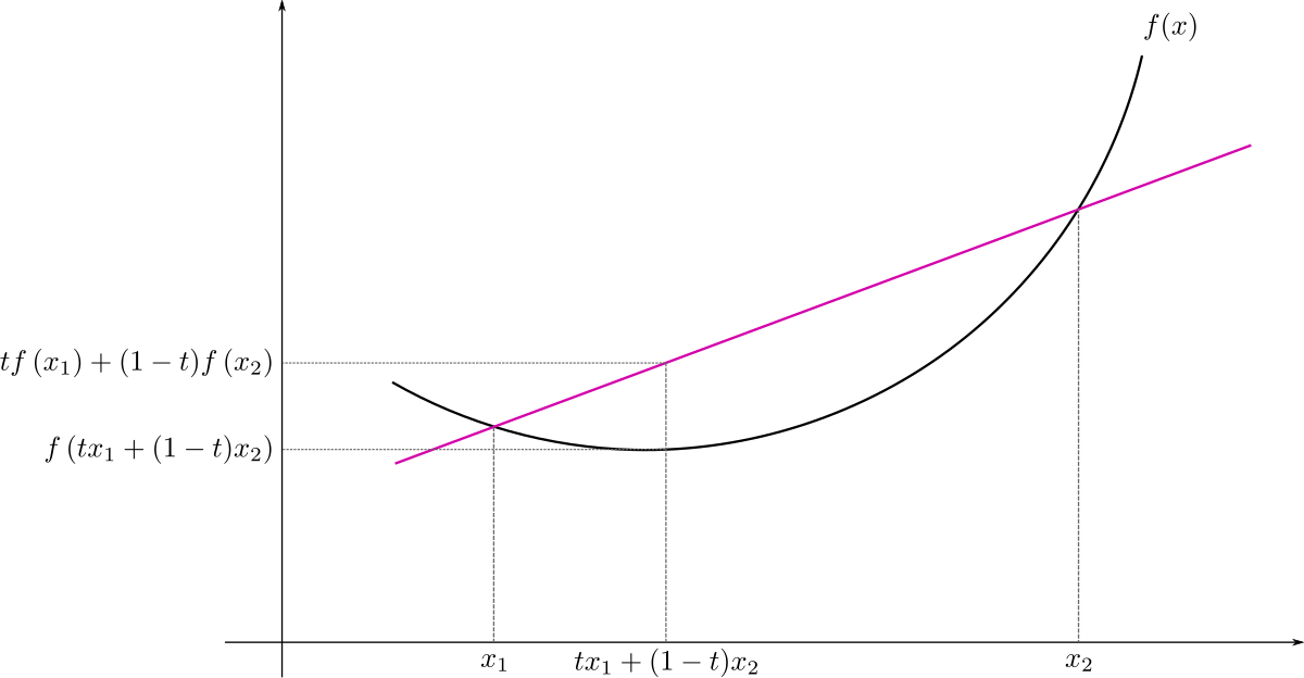
A function $f$ is a convex function if domain of $f$ is a convex set, and the line segment between the points $(x, f(x))$ and $(y, f(y))$ lie above the graph of $f$. Formally, for any $x, y\in \mathrm{dom}(f)$, we have

\[ \underbrace{f(tx + (1-t)y)}_{\text{height of graph of $f$ at a point between $x$ and $y$}} \quad \leq \underbrace{tf(x) + (1-t)f(y)}_{\text{height of point on line segment between $(x, f(x))$ and $(y, f(y))$}},\quad t\in [0, 1] \]

Convex Function: First Order Condition#

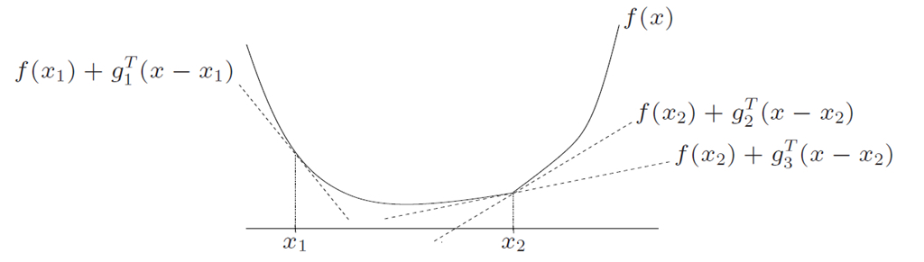
How do we check that a function $f$ is convex? If $f$ is differentiable then $f$ is convex if the graph of $f$ lies above every tangent plane.

Theorem: If $f$ is differentiable then $f$ is convex if and only if for every $x \in \mathrm{dom}(f)$, we have

\[ \underbrace{f(y)}_{\text{height of graph of $f$ over $y$}} \geq \underbrace{f(x) + \nabla f(x)^\top (y - x)}_{\text{height of plane tangent to $f$ at $x$, evaluated over $y$}},\quad \forall y\in \mathrm{dom}(f) \]

Convex Function: Second Order Condition#

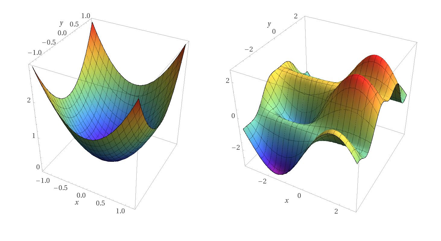
If $f$ is twice-differentiable then $f$ is convex if the “second derivative is positive”.

Theorem: If $f$ is twice-differentiable then $f$ is convex if and only if the Hessian $\nabla^2 f(x)$ is positive semi-definite for every $x\in \mathrm{dom}(f)$.

Properties of Convex Functions#

How to build complex convex functions from simple convex functions:

if $w_1, w_2 \geq 0$ and $f_1, f_2$ are convex, then $h = w_1 f_1 + w_2 f_2$ is convex
if $f$ and $g$ are convex, and $g$ is univariate and non-decreasing then $h = g \circ f$ is convex
Log-sum-exp functions are convex: $f(x) = \log \sum_{k=1}^K e^{x}$

Note: there are many other convexity preserving operations on functions.

Convex Optimization#

A convex optimization problem is an optimization of the following form:

\[\begin{split}\begin{aligned} \mathrm{min}\; &f(x) & (\text{convex objective function})\\ \text{subject to}\; & h_i(x) \leq 0, i=1, \ldots, i & (\text{convex inequality constraints}) \\ & a_j^\top x - b_j = 0, j=1, \ldots, J & (\text{affine equality constraints}) \\ \end{aligned}\end{split}\]

The set of points that satisfy the constraints is called the feasible set.

You can prove that the a convex optimization problem optimizes a convex objective function over a convex feasible set. But why should we care about convex optimization problems?

Theorem: Let $f$ be a convex function defined over a convex feasible set $\Omega$. Then if $f$ has a local minimum at $x\in \Omega$ – $f(y) \geq f(x)$ for $y$ in a small neighbourhood of $x$ – then $f$ has a global minimum at $x$.

Corollary: Let $f$ be a differentiable convex function:

if $f$ is unconstrained, then $f$ has a local minimum and hence global minimum at $x$ if $\nabla f(x) = 0$.
if $f$ is constrained by equalities, then $f$ has a global minimum at $x$ if $\nabla J(x, \lambda) = 0$, where $J(x, \lambda)$ is the Lagrangian of the constrained optimization problem.

Going deeper: Aside

Note: we can also characterize the global minimum of inequalities constrained convex optimization problems using the Lagrangian, but the formulation is more complicated.

Convexity of the Logistic Regression Negative Log-Likelihood#

But why do we care about convex optimization problems? Let’s connect the theory of convex optimization to MLE inference for logistic regression. Recall that the negative log-likelihood of the logistic regression model is

\[\begin{split}\begin{aligned} -\ell(\mathbf{w}) &= -\sum_{n=1}^N y^{(n)}\,\log\,\mathrm{sigm}(\mathbf{w}^\top \mathbf{x}^{(n)}) + (1 - y^{(n)}) \log (1 -\mathrm{sigm}(\mathbf{w}^\top \mathbf{x}^{(n)}))\\ &=\sum_{n=1}^N y^{(n)} \log(e^0 + e^{\mathbf{w}^\top \mathbf{x}^{(n)}}) + (1 - y^{(n)})(- \mathbf{w}^\top \mathbf{x}^{(n)}) \end{aligned}\end{split}\]

Proposition: The negative log-likelihood of logistic regression $-\ell(\mathbf{w})$ is convex.

What does this mean for gradient descent? If gradient descent finds that $\mathbf{w}^*$ is a stationary point of $-\nabla_{\mathbf{w}}\ell(\mathbf{w})$ then $-\ell(\mathbf{w})$ has a global minimum at $\mathbf{w}^*$. Hence, $\ell(\mathbf{w})$ is maximized at $\mathbf{w}^*$.

Proof of the Proposition: Note that

$- \mathbf{w}^\top \mathbf{x}^{(n)}$ and $(1 - y^{(n)})(- \mathbf{w}^\top \mathbf{x}^{(n)})$ are convex, since they are linear
$\log(e^0 + e^{\mathbf{w}^\top \mathbf{x}^{(n)}})$ is convex since it is the composition of a log-sum-exp function (which is convex) and a convex function $\mathbf{w}^\top \mathbf{x}^{(n)}$
$\sum_{n=1}^N y^{(n)} \log(e^0 + e^{\mathbf{w}^\top \mathbf{x}^{(n)}})$ is convex since it is a nonnegative linear combination of convex functions
$-\ell(\mathbf{w})$ is convex since it is the sum of two convex functions

Going deeper: But Does It Always Converge?

We’ve seen that if we choose the learning rate to be too large (say for example 1e10 then gradient descent can fail to converge even if the function $f$ is convex. But how large is “too large”. There are two cases to consider

You have some prior knowledge about how smooth the function $f$ is – i.e. how quickly $f$ can increase or decrease. Then using this you can choose a learning rate that will provably guarantee convergence
In most cases, the objective function (like the log-likelihood) may be too complex to reason about. In which case,
1. we do a scientific “guess-and-check” to determine the learning rate:
  1. we find a learning rate that is large enough to cause gradient descent to diverge
  2. we find a learning rate that is small enough to cause gradient descent to converge too slowly
  3. we choose a range of values between the large rate and the small rate and try them all to determine the optimal rate
2. alternatively, we can choose the step-size $\eta$ adaptively (e.g. when the gradient is large we can set $\eta$ to be moderate to small and when the gradient is small we can set $\eta$ to be larger). There are a number of adaptive step-size regimes that you may want to look up and implement for your specific problem.

The prior knowledge required to choose $\eta$ for provable convergence is called Lipschitz continuity. If we knew that $f$ is convex, differentiable and that there is a constant $L>0$ such that $\|\nabla f(x) - \nabla f(y)\|_2 \leq L\|x -y\|_2$, then if we choose a fixed step size to be $\eta \leq \frac{1}{L}$ then gradient descent provably converges to the global minimum of $f$ as the number of iterations $N$ goes to infinity. The constant $L$ is called the Lipschitz constant.

But How Quickly Can We Get There? Just because we know gradient descent will converge it doesn’t mean that it will give us a good enough approximation of the global minimum within our time limit. This is why studying the rate of convergence of gradient descent is extremely important. Again there are two cases to consider

You have prior knowledge that $f$ is convex, differentiable and its Lipschitz constant is $L$ and suppose that $f$ has a global minimum at $x^*$, then for gradient descent to get within $\epsilon$ of $f(x^*)$, we need $O(1/\epsilon)$ number of iterations.
In most cases, the objective function will fail to be convex and its Lipschitz constant may be too difficult to compute. In this case, we simply stop the gradient descent when the gradient is sufficiently small.

But Does It Scale?#

Gradient is such a simple algorithm that can be applied to any optimization problem for which you can compute the gradient of the objective function.

Question: Does this mean that maximum likelihood inference for statistical models is now an easy task (i.e. just use gradient descent)?

For every likelihood optimization problem, evaluating the gradient at a set of parameters $\mathbf{w}$ requires evaluating the likelihood of the entire dataset using $\mathbf{w}$:

\[ \nabla_{\mathbf{w}} \ell(\mathbf{w}) = -\sum_{n=1}^N \left(y^{(n)} - \frac{1}{1 + e^{-\mathbf{w}^\top\mathbf{x}^{(n)}}} \right) \mathbf{x}^{(n)} =\mathbf{0} \]

Imagine if the size of your dataset $N$ is in the millions. Naively evaluating the gradient just once may take up to seconds or minutes, thus running gradient descent until convergence may be unachievable in practice!

Idea: Maybe we don’t need to use the entire data set to evaluate the gradient during each step of gradient descent. Maybe we can approximate the gradient at $\mathbf{w}$ well enough with just a subset of the data.

15.4. Summary#

For a set of observations $y$, we can collect additional data $x$ and model the conditional distribution $p(Y|X)$. This is exactly regression and classification models do, they use covariates $x$ to predict the outcome $y$.

(Conditional Models) Why do we need additional data $x$? Why isn’t it sufficient to just model $y$ as a binomial, Gaussian or a mixture of Gaussians?
- to predict
- to explain
- to model finer grain variations in y
(Classification) For binary data (like whether or not an individual has kidney cancer), we can model $p(Y|X)$ as a Bernoulli

\[ Y^{(n)} \sim Ber\left(\mathrm{sigm}\left(f\left(\mathbf{X}^{(n)}; \mathbf{w}\right)\right)\right). \]

Geometrically, $f\left(\mathbf{X}^{(n)}; \mathbf{w}\right)$ gives the distance from a decision boundary that separates $y=1$ from $y=0$, and we convert this distance into a probability using the sigmoid function $\mathrm{sigm}$.

(Maximizing the Likelihood) We want to maximize the log Bernoulli likelihood of $y$ (conditioned on $x$) over model parameters $\mathbf{w}$, but the zeros of the gradient of the log-likelihood cannot be analytically solved for!

\[ \nabla_{\mathbf{w}} \ell(\mathbf{w}) = -\sum_{n=1}^N \left(y^{(n)} - \frac{1}{1 + e^{-\mathbf{w}^\top\mathbf{x}^{(n)}}} \right) \mathbf{x}^{(n)} =\mathbf{0} \]

But just because we can’t analytically find the zeros of the gradient, it doesn’t mean that the gradient is useless! The gradient of a loss function points to the direction of the greatest rate of increase, hence the negative gradient points to the direction of the fastest way of decreasing the loss function.

When we iteratively decrease the loss function by changing $\mathbf{w}$ in the direction of the negative gradient, this is called gradient descent.
(Properties of Gradient Descent) Gradient descent sounds like we can optimize any function without work, is it as good as it sounds?
- What do I need to know in order to use gradient descent?
- Is gradient descent guaranteed to converge?
- Is gradient descent efficient?
  - EM was also an algorithm to maximize a log pdf. What is the difference between EM and gradient descent? What was the point of learning EM if we could have just learned gradient descent?
(The Challenges of Conditional Models) Conditional models have so much potential to generate scientific understanding of our data but they are also the most frequently misused!

Suppose that you fit a logistic regression model to predict whether a loan application should be approved. Suppose that you have three covariates:

x_1 representing gender: 0 for male, 1 for female
x_2 for the income
x_3 for the loan amount

Suppose that the parameters you found are:

\[ p(y=1 | x_1, x_2, x_3) = \mathrm{sigm}(-1 + 3 x_1 + 1.5 x_2 + 1.75 x_3). \]

What can I conclude about the loan decisions data that this model was fitted on? Can I deploy this model for usage?
- Bias in your conclusions is exponentially exacerbated by bias in the data collection process.
  - What information are you asking for? If you ask the wrong question, the covariates you collect are at best unpredictive, and at worse they can mask the signal in the data.
    
    In many data collection processes, one finds that the questionnaire might be using “sex” and “gender” interchangeably, or “race” and “ethnicity” interchangeably. But the former (depending on field and context) frequently refers to biological invariants (like chromosomes and genetic lineage), whereas the latter frequently refers to lived experiences (related to identity, culture etc). Caveat: although we collect data on race and sex as if delineation in these categories are more “immutable” or “factual”, many have/do argue that these concepts are also social constructs (see discussion on false binaries and false aggregation)!
    
    When you ask for “sex” are you asking about a person’s chromosomal information, because you’re studying chromosomal related diseases, or are you asking about their experiences with the US medical system and how their health outcome is affected by their gender identity OR the identity that people tend to assume of them? For example: women, especially women of color, tend to be under-diagnosed and mis-diagnosed due to gendered treatments of patients.
    
    To complicate matters, the terms “gender” and “sex” can have very specific legal definitions – that may not align with definitions in medical or sociological contexts! For example, the language of the Equal Credit Opportunity Act is written in terms of “sex”, however, this term is not defined in the ECOA. The Consumer Financial Protection Bureau interprets (in their operating philosophy) this term to include both sexual orientation and gender identity.
  - Did you already bias the answer? If you gave confusing, misleading or incorrect options for answers, then the covariates you collect are at best unpredictive, and at worse they can mask the signal in the data.
    
    In many data collection processes, one finds that the respondent is forced into a category that is unrepresentative of their experience, like having “Asian” as a broad racial category that includes South Asian, East Asian, South East Asian, like providing binary choices for gender or sex.
    
    If you are looking for disparities in health outcomes, you might miss disparities amongst important smaller subgroups within broad group of “Asian”, since health outcomes are often affected by income and Asian-Americans have the largest in-group income disparity.
  - Should you be asking for this information? The complexity of asking a seemingly simple question can seem overwhelming, often we resort to over-collecting (collecting every piece of information that we can think of) or under-collecting (not collecting any sensitive attribute).
    
    Why you might not want to But respondents (e.g. patients, applicants for benefits) can be suspicious that their data can be used precisely to discriminate against them on the basis of protected attributes. Note that data collection have often historically been used to oppress, not to up-lift, vulnerable communities. So collecting this data without clear purpose can compromise user trust and constitute a privacy threat if this data is not well protected.
    
    Why you should However, in order to make sure our model is not disproportionately negatively impacting vulnerable subgroups and that we are in compliance with laws like the EOCA, we need to check for disparate impact on protected groups. But in order to do that, we need to have access to sensitive attributes.
- Is correlation causation?
  - It appears that the sex of the applicant the logistic regression model has the greatest influence on the prediction of the model, does this mean that the human decision makers were biased? (Hint: not necessarily, but it might be a hypothesis to explore to retroactively detect potential regulatory violation in this dataset.)
  - If the interpretations of the coefficients of the logistic regression model does not imply human bias in the data, then can we use this model for real life loan decisions? (Hint: the answer is NO. It would be an violation!)

15.5. Further Reading#

Gradient Descent and Stochastic Gradient Descent

(Introductory) Gradient Descent Algorithm and Its Variants
(In-Depth) Stochastic Gradient “Descent” Algorithm
(Advanced) On the Convergence of Stochastic Gradient Descent with Adaptive Stepsizes
(Advanced) On the Stability and Convergence of Stochastic Gradient Descent with Momentum
(Practical) Stochastic Gradient Descent Tricks
(In-Depth) Convex Optimization and Approximation

Logistic Regression and Gradient Descent

Contents

15. Logistic Regression and Gradient Descent#

15.1. Logistic Regression#

Coin-Toss Revisited: Modeling a Bernoulli Variable with Covariates#

The Logistic Regression Model#

Interpreting a Logistic Regression Model#

With Great Explanatory Power Comes Great Responsibility!#

When not to use sensitive/protected attributes#

When you might want to use sensitive/protected attributes#

Appropriate usage of sensitive/protected attributes#

Maximizing the Logistic Regression Log-likelihood#

15.2. Gradient Descent#

Gradient as Directional Information#

An Intuition for Gradient Descent#

Gradient Descent: the Algorithm#

Diagnosing Design Choices with the Trajectory#

Diagnosing Issues with the Trajectory#

Gradient Descent: Step Size Matters#

Gradient Descent for Logistic Regression#

But Did We Optimize It?#

15.3. Convex Optimization#

Convex Sets#

Convex Functions#

Convex Function: First Order Condition#

Convex Function: Second Order Condition#

Properties of Convex Functions#

Convex Optimization#

Convexity of the Logistic Regression Negative Log-Likelihood#

But Does It Scale?#

15.4. Summary#

15.5. Further Reading#