Lab 7: Non-Linear Models for Regression#
This lab is adapted from AM207 (Harvard). Data files are in the book’s data/ folder. Worked solutions are collapsed: try each exercise before expanding them.
class Feedforward:
    def __init__(self, architecture, random=None, weights=None):
        self.params = {'H': architecture['width'],
                       'L': architecture['hidden_layers'],
                       'D_in': architecture['input_dim'],
                       'D_out': architecture['output_dim'],
                       'activation_type': architecture['activation_fn_type'],
                       'activation_params': architecture['activation_fn_params']}

        self.D = (  (architecture['input_dim'] * architecture['width'] + architecture['width'])
                  + (architecture['output_dim'] * architecture['width'] + architecture['output_dim'])
                  + (architecture['hidden_layers'] - 1) * (architecture['width']**2 + architecture['width'])
                 )

        if random is not None:
            self.random = random
        else:
            self.random = np.random.RandomState(0)

        self.h = architecture['activation_fn']

        if weights is None:
            self.weights = self.random.normal(0, 1, size=(1, self.D))
        else:
            self.weights = weights

        self.objective_trace = np.empty((1, 1))
        self.weight_trace = np.empty((1, self.D))


    def forward(self, weights, x):
        ''' Forward pass given weights and input '''
        H = self.params['H']
        D_in = self.params['D_in']
        D_out = self.params['D_out']

        assert weights.shape[1] == self.D

        if len(x.shape) == 2:
            assert x.shape[0] == D_in
            x = x.reshape((1, D_in, -1))
        else:
            assert x.shape[1] == D_in

        weights = weights.T


        #input to first hidden layer
        W = weights[:H * D_in].T.reshape((-1, H, D_in))
        b = weights[H * D_in:H * D_in + H].T.reshape((-1, H, 1))
        input = self.h(np.matmul(W, x) + b)
        index = H * D_in + H

        assert input.shape[1] == H

        #additional hidden layers
        for _ in range(self.params['L'] - 1):
            before = index
            W = weights[index:index + H * H].T.reshape((-1, H, H))
            index += H * H
            b = weights[index:index + H].T.reshape((-1, H, 1))
            index += H
            output = np.matmul(W, input) + b
            input = self.h(output)

            assert input.shape[1] == H

        #output layer
        W = weights[index:index + H * D_out].T.reshape((-1, D_out, H))
        b = weights[index + H * D_out:].T.reshape((-1, D_out, 1))
        output = np.matmul(W, input) + b
        assert output.shape[1] == self.params['D_out']

        return output

    def make_objective(self, x_train, y_train, reg_param=None):
        ''' Make objective functions: depending on whether or not you want to apply l2 regularization '''

        if reg_param is None:

            def objective(W, t):
                squared_error = np.linalg.norm(y_train - self.forward(W, x_train), axis=1)**2
                sum_error = np.sum(squared_error)
                return sum_error

            return objective, grad(objective)

        else:

            def objective(W, t):
                squared_error = np.linalg.norm(y_train - self.forward(W, x_train), axis=1)**2
                mean_error = np.mean(squared_error) + reg_param * np.linalg.norm(W)
                return mean_error

            return objective, grad(objective)

    def fit(self, x_train, y_train, params, reg_param=None):
        ''' Wrapper for MLE through gradient descent '''
        assert x_train.shape[0] == self.params['D_in']
        assert y_train.shape[0] == self.params['D_out']

        ### make objective function for training
        self.objective, self.gradient = self.make_objective(x_train, y_train, reg_param)

        ### set up optimization
        step_size = 0.01
        max_iteration = 5000
        check_point = 100
        weights_init = self.weights.reshape((1, -1))
        mass = None
        optimizer = 'adam'
        random_restarts = 5

        if 'step_size' in params.keys():
            step_size = params['step_size']
        if 'max_iteration' in params.keys():
            max_iteration = params['max_iteration']
        if 'check_point' in params.keys():
            self.check_point = params['check_point']
        if 'init' in params.keys():
            weights_init = params['init']
        if 'call_back' in params.keys():
            call_back = params['call_back']
        if 'mass' in params.keys():
            mass = params['mass']
        if 'optimizer' in params.keys():
            optimizer = params['optimizer']
        if 'random_restarts' in params.keys():
            random_restarts = params['random_restarts']

        def call_back(weights, iteration, g):
            ''' Actions per optimization step '''
            objective = self.objective(weights, iteration)
            self.objective_trace = np.vstack((self.objective_trace, objective))
            self.weight_trace = np.vstack((self.weight_trace, weights))
            if (iteration % self.check_point == 0) & (iteration > 0):
                print("Iteration {} lower bound {}; gradient mag: {}".format(iteration, objective, np.linalg.norm(self.gradient(weights, iteration))))

        ### train with random restarts
        optimal_obj = 1e16
        optimal_weights = self.weights

        for i in range(random_restarts):
            if optimizer == 'adam':
                adam(self.gradient, weights_init, step_size=step_size, num_iters=max_iteration, callback=call_back)
            local_opt = np.min(self.objective_trace[-100:])

            if local_opt < optimal_obj:
                opt_index = np.argmin(self.objective_trace[-100:])
                self.weights = self.weight_trace[-100:][opt_index].reshape((1, -1))
            weights_init = self.random.normal(0, 1, size=(1, self.D))

        self.objective_trace = self.objective_trace[1:]
        self.weight_trace = self.weight_trace[1:]
Problem Description: Non-linear Models for Regression#
From Chapter 21, we’ve seen that we can take our favourite generalized linear models and replace the linear function \(\mathbf{w}^\top \mathbf{X}\) with \(g_{\mathbf{W}}(\mathbf{X})\), where \(g_{\mathbf{W}}\) is a neural network with parameters \(\mathbf{W}\). The advantage of using neural networks to represent non-linear function is that neural networks allows us to build up complex non-linear functions very cheaply and quickly through composition of simple functions. A neural network \(g_{\mathbf{W}}\) with a fixed architecture can approximate a wide range of different functions.
In this lab, we compare fitting neural networks regression models with polynomial regression models.
Part I. Small Data Set#
Read in the data in lab_7_data.csv.
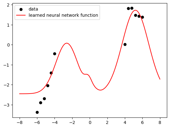
(Learning the Model) Fit 100 different MLE neural network models (with the given architecture or your own choice) on this data. The data is small so don’t bootstrap, rather, initialize your network parameters randomly for each fit.
(Model Evaluation) Compute the average log-likelihood of the observed data over these 100 MLE models.
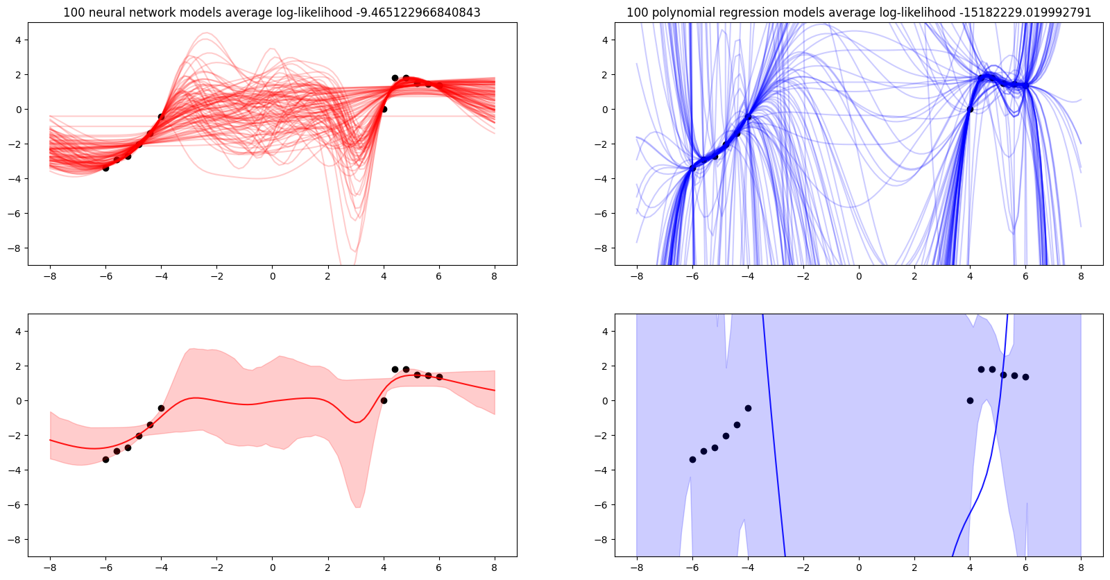
(Model Evaluation) Visualize the predictive distributions of your 100 MLE models (i.e. use them to predict on a range of uniformly spaced values from [-8, 8] and then plot either the 95% predictive interval or plot all the models as lines).
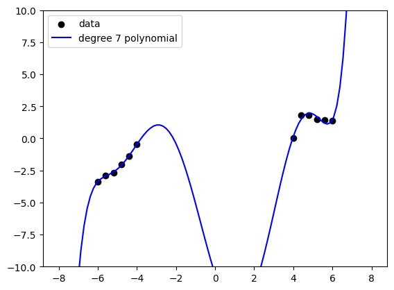
(Compare with Polynomial Regression) Do the above for polynomial models with polynomial degree 7. Which model class (polynomial or neural network) is a better fit for the data? Which model class produces better aleatoric uncertainty? Which model class produces better epistemic uncertainty? Why?
| x | y | |
|---|---|---|
| 0 | -6.0 | -3.380284 |
| 1 | -5.6 | -2.892117 |
| 2 | -5.2 | -2.690059 |
| 3 | -4.8 | -2.040000 |
| 4 | -4.4 | -1.399942 |
Solution: Part I
Example of Fitting One NN to the Data
###define design choices in gradient descent
params = {'step_size':1e-3,
          'max_iteration':4000,
          'random_restarts':1,
          'check_point':200}

#fit my neural network to minimize MSE on the given data
nn.fit(x.reshape((1, -1)), y.reshape((1, -1)), params)
Iteration 200 lower bound 49.42633385370296; gradient mag: 28.316275482037554
Iteration 400 lower bound 46.64774569354082; gradient mag: 13.477552540546968
Iteration 600 lower bound 45.25067576634001; gradient mag: 8.65493225556682
Iteration 800 lower bound 26.977925085924856; gradient mag: 20.354176994190933
Iteration 1000 lower bound 22.02986716940496; gradient mag: 17.427416991221946
Iteration 1200 lower bound 18.434367471681036; gradient mag: 15.092044558814079
Iteration 1400 lower bound 15.673763205688546; gradient mag: 13.076506887891876
Iteration 1600 lower bound 13.511041180892445; gradient mag: 11.2926913337729
Iteration 1800 lower bound 11.80461440400386; gradient mag: 9.707342852428727
Iteration 2000 lower bound 10.452003162028157; gradient mag: 8.324954075223918
Iteration 2200 lower bound 9.360728932888753; gradient mag: 7.221146412450926
Iteration 2400 lower bound 8.41037187354601; gradient mag: 6.6270219395874035
Iteration 2600 lower bound 7.471807925987624; gradient mag: 6.054967192028712
Iteration 2800 lower bound 6.657649714610487; gradient mag: 5.301596015489049
Iteration 3000 lower bound 5.932348941430827; gradient mag: 4.738230196194092
Iteration 3200 lower bound 5.261275455408112; gradient mag: 4.278187646372163
Iteration 3400 lower bound 4.631006056116021; gradient mag: 3.893374295011206
Iteration 3600 lower bound 4.038157311705765; gradient mag: 3.556269206709464
Iteration 3800 lower bound 3.486418190371086; gradient mag: 3.2444781370885587
x_test = np.linspace(-8, 8, 100)

#predict on x_test
y_test = nn.forward(nn.weights, x_test.reshape((1, -1)))

#visualize our learned model
plt.scatter(x, y, color='black', label='data')
plt.plot(x_test, y_test.flatten(), color='red', label='learned neural network function')
plt.legend(loc='best')
plt.show()
Example of Fitting One Polynomial Regression Model to the Data
#set up for polynomial (deg 7) regression
linear_model = LinearRegression()
poly = PolynomialFeatures(7)

#fit a polynomial model
x_poly = poly.fit_transform(x.reshape((-1, 1)))
x_test_poly = poly.fit_transform(x_test.reshape((-1, 1)))
linear_model.fit(x_poly, y)

#predict on x_test
y_test_poly = linear_model.predict(x_test_poly)

#visualize our learned model
plt.scatter(x, y, color='black', label='data')
plt.plot(x_test, y_test_poly.flatten(), color='blue', label='degree 7 polynomial')
plt.legend(loc='best')
plt.ylim([-10, 10])
plt.show()
Fitting Multiple Models to the Data Through Bootstrapping and Random Restarts
##define normal log-likelihood with variance 0.5**2
output_noise = 0.5**2
log_likelihood = lambda y_actual, y_pred: -0.5 * len(y_actual.flatten()) * np.log(2 * np.pi * output_noise) - 0.5 * ((y_actual.flatten() - y_pred.flatten())**2).sum() / output_noise

trials = 100

y_test_nn = []
y_test_poly = []
log_lkhd_nn = []
log_lkhd_poly = []

for i in range(trials):
    if i % 10 == 0:
        print('trial:', i)

    #generate a bootstrap sample from the data
    indices = np.random.choice(np.arange(len(x)), size=len(x))
    bootstrap_x = x[indices]
    bootstrap_y = y[indices]

    #fit neural network
    ###define design choices in gradient descent
    random = np.random.RandomState(i)
    params = {'step_size':1e-3,
              'max_iteration':3000,
              'random_restarts':1,
              'check_point':3000,
              'init': random.normal(0, 1, size=nn.weights.shape)
              }

    #reset the optimization traces kept by the previous fit
    nn.objective_trace = np.empty((1, 1))
    nn.weight_trace = np.empty((1, nn.D))
    #fit my neural network to minimize MSE on the given data
    nn.fit(x.reshape((1, -1)), y.reshape((1, -1)), params)
    #predict on x_test
    y_test = nn.forward(nn.weights, x_test.reshape((1, -1))).flatten()
    y_test_nn.append(y_test)

    #compute log likelihood on observed data
    y_train = nn.forward(nn.weights, x.reshape((1, -1))).flatten()
    log_lkhd_nn.append(log_likelihood(y, y_train))

    #fit a polynomial model
    bootstrap_x_poly = poly.fit_transform(bootstrap_x.reshape((-1, 1)))
    bootstrap_x_test_poly = poly.fit_transform(x_test.reshape((-1, 1)))
    linear_model.fit(bootstrap_x_poly, bootstrap_y)

    #predict on x_test
    y_test = linear_model.predict(x_test_poly)
    y_test_poly.append(y_test)

    #compute log likelihood on observed data
    y_train = linear_model.predict(x_poly)
    log_lkhd_poly.append(log_likelihood(y, y_train.flatten()))
trial: 0
trial: 10
trial: 20
trial: 30
trial: 40
trial: 50
trial: 60
trial: 70
trial: 80
trial: 90
fig, ax = plt.subplots(2, 2, figsize=(20, 10))
ax[0, 0].scatter(x, y, color='black', label='data')
ax[0, 1].scatter(x, y, color='black', label='data')
ax[1, 0].scatter(x, y, color='black', label='data')
ax[1, 1].scatter(x, y, color='black', label='data')

#plot the neural network and polynomial models
for y_nn, y_poly in zip(y_test_nn, y_test_poly):
    ax[0, 0].plot(x_test, y_nn.flatten(), color='red', alpha=0.2)
    ax[0, 1].plot(x_test, y_poly, color='blue', alpha=0.2)

#compute 95% predictive interval
y_test_nn = np.array(y_test_nn)
y_test_poly = np.array(y_test_poly)

y_test_nn_ub = np.percentile(y_test_nn, 97.5, axis=0)
y_test_nn_mean = y_test_nn.mean(axis=0)
y_test_nn_lb = np.percentile(y_test_nn, 2.5, axis=0)

y_test_poly_ub = np.percentile(y_test_poly, 97.5, axis=0)
y_test_poly_mean = y_test_poly.mean(axis=0)
y_test_poly_lb = np.percentile(y_test_poly, 2.5, axis=0)

#plot 95% predictive interval
ax[1, 0].fill_between(x_test, y_test_nn_ub, y_test_nn_lb, color='red', alpha=0.2)
ax[1, 1].fill_between(x_test, y_test_poly_ub, y_test_poly_lb, color='blue', alpha=0.2)
ax[1, 0].plot(x_test, y_test_nn_mean, color='red', alpha=0.9)
ax[1, 1].plot(x_test, y_test_poly_mean, color='blue', alpha=0.9)
ax[1, 0].set_ylim([-9, 5])
ax[1, 1].set_ylim([-9, 5])

ax[0, 0].set_title('{} neural network models average log-likelihood {}'.format(trials, np.mean(log_lkhd_nn)))
ax[0, 1].set_title('{} polynomial regression models average log-likelihood {}'.format(trials, np.mean(log_lkhd_poly)))
ax[0, 0].set_ylim([-9, 5])
ax[0, 1].set_ylim([-9, 5])
plt.show()
Not covered here: which model class fits the data better, and which gives better aleatoric and epistemic uncertainty.
Part II. “Large” Data Set#
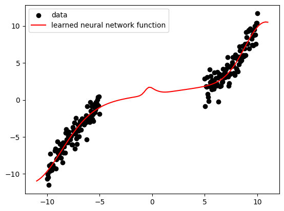
Using the data that is generated by the code provided below.
(Learning the Model) Fit 100 different MLE neural network models (with the given architecture or your own choice) on this data. Bootstrap from the data as well as initialize your network parameters randomly for each fit.
(Model Evaluation) Compute the average log-likelihood of the observed data over these 100 MLE models.
(Model Evaluation) Visualize the predictive distributions of your 100 MLE models (i.e. use them to predict on a range of uniformly spaced values from [-11, 11] and then plot either the 95% predictive interval or plot all the models as lines).
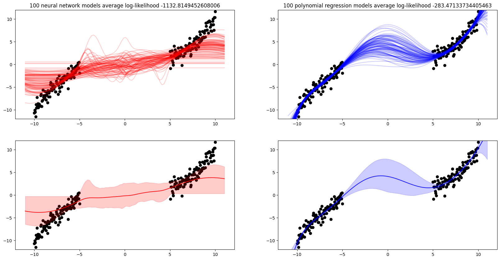
(Compare with Polynomial Regression) Do the above for polynomial models with polynomial degree 7. Which model class (polynomial or neural network) is a better fit for the data? Which model class produces better aleatoric uncertainty? Which model class produces better epistemic uncertainty? Why?
Solution: Part II
Example of Fitting One NN to the Data
###define design choices in gradient descent
params = {'step_size':1e-2,
          'max_iteration':5000,
          'random_restarts':1,
          'check_point': 200}

#fit my neural network to minimize MSE on the given data
nn.fit(x.reshape((1, -1)), y.reshape((1, -1)), params)
Iteration 200 lower bound 999.8560933313968; gradient mag: 407.0821635820762
Iteration 400 lower bound 494.17182191658884; gradient mag: 180.36779470311583
Iteration 600 lower bound 340.25643791287155; gradient mag: 95.5977574866079
Iteration 800 lower bound 278.17348297852925; gradient mag: 58.86499619405767
Iteration 1000 lower bound 246.21307401089638; gradient mag: 39.52482717272701
Iteration 1200 lower bound 228.83226738193153; gradient mag: 26.79886111518004
Iteration 1400 lower bound 219.65143818913631; gradient mag: 18.29872158092852
Iteration 1600 lower bound 214.74429144704607; gradient mag: 12.884314783056643
Iteration 1800 lower bound 211.9271061647745; gradient mag: 9.55600312099037
Iteration 2000 lower bound 210.11132277844064; gradient mag: 20.664696144655817
Iteration 2200 lower bound 208.78627802738816; gradient mag: 6.285293507854829
Iteration 2400 lower bound 207.71694159106613; gradient mag: 5.482096767838978
Iteration 2600 lower bound 206.8091063642461; gradient mag: 4.812070137393829
Iteration 2800 lower bound 206.0138259043366; gradient mag: 15.774844878422039
Iteration 3000 lower bound 205.31103226667273; gradient mag: 66.86364733424382
Iteration 3200 lower bound 204.67335459852512; gradient mag: 36.37408257061808
Iteration 3400 lower bound 204.101527911743; gradient mag: 45.72419327390756
Iteration 3600 lower bound 203.58044872223633; gradient mag: 18.54338426864378
Iteration 3800 lower bound 203.11501061829952; gradient mag: 98.23503708714452
Iteration 4000 lower bound 202.7580566956953; gradient mag: 333.03625611355216
Iteration 4200 lower bound 202.2677631836354; gradient mag: 2.4415967308734383
Iteration 4400 lower bound 201.89890611071505; gradient mag: 2.143542293326703
Iteration 4600 lower bound 201.55711138616232; gradient mag: 2.433805625325038
Iteration 4800 lower bound 201.23921079885133; gradient mag: 2.58391161742893
x_test = np.linspace(-11, 11, 100)

#predict on x_test
y_test = nn.forward(nn.weights, x_test.reshape((1, -1)))

#visualize our learned model
plt.scatter(x, y, color='black', label='data')
plt.plot(x_test, y_test.flatten(), color='red', label='learned neural network function')
plt.legend(loc='best')
plt.show()
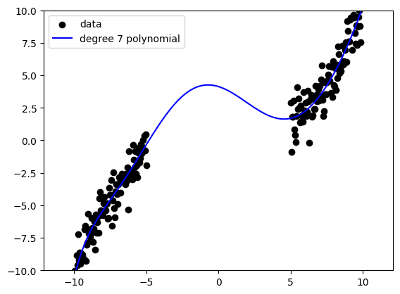
Example of Fitting One Polynomial Regression Model to the Data
#set up for polynomial (deg 7) regression
linear_model = LinearRegression()
poly = PolynomialFeatures(7)

#fit a polynomial model
x_poly = poly.fit_transform(x.reshape((-1, 1)))
x_test_poly = poly.fit_transform(x_test.reshape((-1, 1)))
linear_model.fit(x_poly, y)

#predict on x_test
y_test_poly = linear_model.predict(x_test_poly)

#visualize our learned model
plt.scatter(x, y, color='black', label='data')
plt.plot(x_test, y_test_poly.flatten(), color='blue', label='degree 7 polynomial')
plt.legend(loc='best')
plt.ylim([-10, 10])
plt.show()
##define normal log-likelihood with the noise variance of the data
output_noise = y_var
log_likelihood = lambda y_actual, y_pred: -0.5 * len(y_actual.flatten()) * np.log(2 * np.pi * output_noise) - 0.5 * ((y_actual.flatten() - y_pred.flatten())**2).sum() / output_noise

trials = 100

y_test_nn = []
y_test_poly = []
log_lkhd_nn = []
log_lkhd_poly = []

for i in range(trials):
    if i % 10 == 0:
        print('trial:', i)

    #generate a bootstrap sample from the data
    indices = np.random.choice(np.arange(len(x)), size=len(x))
    bootstrap_x = x[indices]
    bootstrap_y = y[indices]

    #fit neural network
    ###define design choices in gradient descent
    random = np.random.RandomState(i)
    params = {'step_size':1e-3,
              'max_iteration':3000,
              'random_restarts':1,
              'check_point':3000,
              'init': random.normal(0, 1, size=nn.weights.shape)
              }

    #reset the optimization traces kept by the previous fit
    nn.objective_trace = np.empty((1, 1))
    nn.weight_trace = np.empty((1, nn.D))
    #fit my neural network to minimize MSE on the bootstrap sample
    nn.fit(bootstrap_x.reshape((1, -1)), bootstrap_y.reshape((1, -1)), params)
    #predict on x_test
    y_test = nn.forward(nn.weights, x_test.reshape((1, -1))).flatten()
    y_test_nn.append(y_test)

    #compute log likelihood on observed data
    y_train = nn.forward(nn.weights, x.reshape((1, -1))).flatten()
    log_lkhd_nn.append(log_likelihood(y, y_train))

    #fit a polynomial model
    bootstrap_x_poly = poly.fit_transform(bootstrap_x.reshape((-1, 1)))
    bootstrap_x_test_poly = poly.fit_transform(x_test.reshape((-1, 1)))
    linear_model.fit(bootstrap_x_poly, bootstrap_y)

    #predict on x_test
    y_test = linear_model.predict(x_test_poly)
    y_test_poly.append(y_test)

    #compute log likelihood on observed data
    y_train = linear_model.predict(x_poly)
    log_lkhd_poly.append(log_likelihood(y, y_train.flatten()))
trial: 0
trial: 10
trial: 20
trial: 30
trial: 40
trial: 50
trial: 60
trial: 70
trial: 80
trial: 90
fig, ax = plt.subplots(2, 2, figsize=(20, 10))
ax[0, 0].scatter(x, y, color='black', label='data')
ax[0, 1].scatter(x, y, color='black', label='data')
ax[1, 0].scatter(x, y, color='black', label='data')
ax[1, 1].scatter(x, y, color='black', label='data')

#plot the neural network and polynomial models
for y_nn, y_poly in zip(y_test_nn, y_test_poly):
    ax[0, 0].plot(x_test, y_nn.flatten(), color='red', alpha=0.2)
    ax[0, 1].plot(x_test, y_poly, color='blue', alpha=0.2)

#compute 95% predictive interval
y_test_nn = np.array(y_test_nn)
y_test_poly = np.array(y_test_poly)

y_test_nn_ub = np.percentile(y_test_nn, 97.5, axis=0)
y_test_nn_mean = y_test_nn.mean(axis=0)
y_test_nn_lb = np.percentile(y_test_nn, 2.5, axis=0)

y_test_poly_ub = np.percentile(y_test_poly, 97.5, axis=0)
y_test_poly_mean = y_test_poly.mean(axis=0)
y_test_poly_lb = np.percentile(y_test_poly, 2.5, axis=0)

#plot 95% predictive interval
ax[1, 0].fill_between(x_test, y_test_nn_ub, y_test_nn_lb, color='red', alpha=0.2)
ax[1, 1].fill_between(x_test, y_test_poly_ub, y_test_poly_lb, color='blue', alpha=0.2)
ax[1, 0].plot(x_test, y_test_nn_mean, color='red', alpha=0.9)
ax[1, 1].plot(x_test, y_test_poly_mean, color='blue', alpha=0.9)
ax[1, 0].set_ylim([-12, 12])
ax[1, 1].set_ylim([-12, 12])

ax[0, 0].set_title('{} neural network models average log-likelihood {}'.format(trials, np.mean(log_lkhd_nn)))
ax[0, 1].set_title('{} polynomial regression models average log-likelihood {}'.format(trials, np.mean(log_lkhd_poly)))
ax[0, 0].set_ylim([-12, 12])
ax[0, 1].set_ylim([-12, 12])
plt.show()
Not covered here: which model class fits the data better, and which gives better aleatoric and epistemic uncertainty.