12. Bayesian Latent Variable Models and Variational Inference

This chapter is adapted from AM207 (Harvard, Fall 2021). Watch the recorded lecture.

In this chapter

1. Bayesian Latent Variable Models

2. Coordinate Ascent Variational Inference

3. Bayesian Gaussian Mixture Models

Show code cell content

Hide code cell content

### Import basic libraries
import numpy as np
import scipy as sp
import pandas as pd
import sklearn as sk
from sklearn.linear_model import LinearRegression
import matplotlib.pyplot as plt
%matplotlib inline

12.1. Bayesian Latent Variable Models

Overfitting is an always a concern when using MLE model parameters. We can mitigate the effect of outliers in the data on the model we learn by treating the parameters as random variables and placing priors on them.

In a latent variable model, maximum likelihood inference treats parameters \(\theta\), \(\phi\) as unknown constants and produces point-estimates for them. In a Bayesian latent variable model, \(\theta\), \(\phi\) are random variables and we derive the posterior distribution over them.

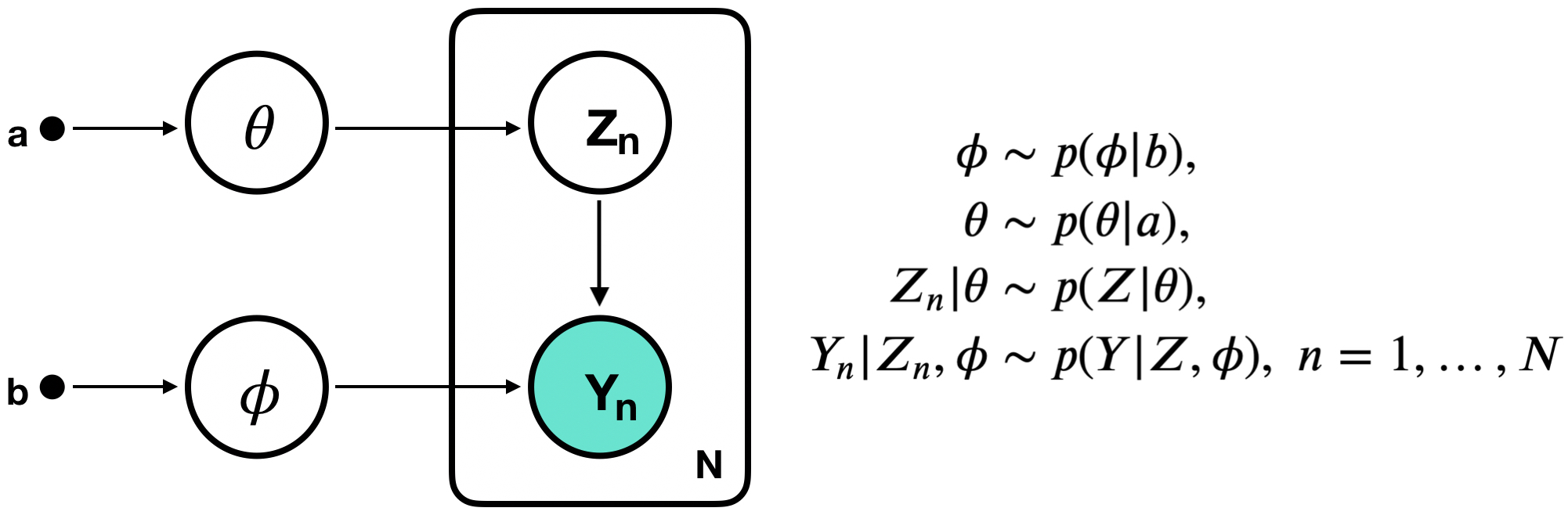
That is, we want to infer

\[p(\theta, \phi, Z_1, \ldots, Z_N|Y_1, \ldots, Y_N, a, b) = \frac{p(\theta | a)p(\phi|b)\prod_{n}p(Y_n|Z_n, \phi)p(Z_n|\theta)}{\prod_{n} p(Y_n)}.\]

Challenges in Bayesian Inference

Unfortunately, most Bayesian models with multiple types of random variables (like Bayesian latent variable models) have complex posteriors that do not match known distributions. Exact inference is not possible.

Sampling from the posterior may not always be the best option because:

1. Convergence of samplers may be slow (due to high dimensionality of the distribution or multimodality)
   
   

2. Samplers like Metropolis-Hastings requires evaluating the likelihood \(\prod_n p(Y_n | Z_n, \phi)\) in each iteration, if the observed data is large (\(N\) is in the millions), this computation is expensive.

The Idea of Variational Inference

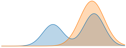
Idea: (Approximate Inference) Approximate the hard posterior \(p(\theta, \phi, Z_1, \ldots, Z_N|Y_1, \ldots, Y_N)\) with a distribution \(q\) that is easy to sample from (like a Gaussian). Any computation involving the posterior can now be done with \(q\).

This approximation of \(p(\theta, \phi, Z_1, \ldots, Z_N|Y_1, \ldots, Y_N)\) with a distribution \(q\) is called variational inference.

The Design of the Variational Objective

Goal: given a target posterior distribution \(p(\psi | Y_1, \ldots, Y_N)\), \(\psi \in \mathbb{R}^I\) we want to find a distribution \(q(\psi |\lambda^*)\) in a family of distributions \(Q = \{q(\psi |\lambda) | \lambda \in \Lambda \}\) such that \(q(\psi |\lambda^*)\) best approximates \(p\).

Design Choices: we need to choose:

A. (Variational family) a family \(Q\) of candidate distributions for approximating \(p\). The members of \(Q\) are called the variational distributions.

Our Choice: we assume that the joint \(q(\psi)\) factorizes completely over each dimension of \(\psi\), i.e. \(q(\psi)= \prod_{i=1}^I q(\psi_i | \lambda_i)\). This is called the mean field assumption. What can go wrong with this design choice?

B. (Divergence measure) a divergence measure to quantify the difference between \(p\) and \(q\).

Our Choice:

\[D_{\text{KL}}(q(\psi | \lambda) \| p(\psi | Y_1, \ldots, Y_N)) = \mathbb{E}_{\psi \sim q(\psi|\lambda)}\left[\log\left( \frac{q(\psi | \lambda)}{p(\psi | Y_1, \ldots, Y_N)} \right) \right]\]

What can go wrong with this design choice?

Variational Inference as Optimization

We now formalize variational inference for a target \(p(\psi)\): find \(q(\psi|\lambda^*)\) where

\[\begin{split}\begin{aligned} \lambda^* &= \underset{\lambda}{\text{argmin}}\; D_{\text{KL}}(q(\psi|\lambda) \| p(\psi|Y_1, \ldots, Y_N))) \\ &= \underset{\lambda}{\text{argmin}}\; \mathbb{E}_{\psi \sim q(\psi|\lambda)}\left[\log\left(\frac{q(\psi | \lambda)}{p(\psi|Y_1, \ldots, Y_N))}\right) \right] \end{aligned}\end{split}\]

Recall that for EM, we had proved that minimizing the KL is equivalent to maximizing the ELBO (for which it is easier to compute the gradient). We will do the same here:

\[\begin{split}\begin{aligned} \underset{\lambda}{\min}D_{\text{KL}}(q(\psi|\lambda) \| p(\psi|Y_1, \ldots, Y_N))) \overset{\text{equiv}}{\equiv}& \underset{\lambda}{\max} -D_{\text{KL}}(q(\psi|\lambda) \| p(\psi|Y_1, \ldots, Y_N))) \\ =& \underset{\lambda}{\max} -\mathbb{E}_{\psi \sim q(\psi|\lambda)}\left[\log\left(\frac{q(\psi | \lambda)}{p(\psi|Y_1, \ldots, Y_N))} \right)\right] \\ =& \underset{\lambda}{\max}\underbrace{\mathbb{E}_{\psi \sim q(\psi|\lambda)}\left[\log\left(\frac{p(\psi, Y_1, \ldots, Y_N))}{q(\psi | \lambda)} \right)\right]}_{ELBO(\lambda)} \\ &- \log p(Y_1, \ldots, Y_N). \end{aligned}\end{split}\]

Thus, the variational objective can be rephrased as maximizing the \(ELBO\).

Gradients of the ELBO

Unfortunately, the ELBO for variational inference of the posterior does not have easy gradients,

\[\begin{aligned} \nabla_{\lambda}\,\underbrace{\mathbb{E}_{\psi \sim q(\psi|\lambda)}\left[\log\left(\frac{p(\psi, Y_1, \ldots, Y_N)}{q(\psi | \lambda)} \right)\right]}_{ELBO(\lambda)}. \end{aligned}\]

In particular, the issue is that the gradient taken is with respect to the parameter \(\psi\) of the distribution over which we are taking the expectation - i.e. we cannot push the gradient into the expectation.

In this chapter, we will maximize the \(ELBO\) using coordinate ascent (just as in the case of EM). But you’ll see that coordinate ascent variational inference requires that we perform model specific computations (often in closed form). This restrict the class of Bayesian models for which we can perform variational inference.

Two of the major developments we will cover in Chapter 22 address how to estimate this gradient efficiently and without bias.

Coordinate Ascent Variational Inference

Going deeper: Aside

Download the derivation (PDF)

Maximizing the ELBO via Coordinate Ascent

The coordinate ascent algorithm maximizes an objective function \(ELBO(\lambda)\) by iteratively maximizing over \(\lambda_i\), holding constant \(\lambda_{-i} = [\lambda_1\; \ldots\; \lambda_{i-1}\; \lambda_{i+1}\; \ldots\; \lambda_{I}]\).

The coordinate ascent variational inference algorithm:

0. Initialization: pick an initial value \(\lambda^{(0)}\)

1. Coordinate-wise maximization:

   Repeat for \(j=1, \ldots, J\) iterations:

   \(\quad\quad\) Cycle thru \(i=1, \ldots, I\) coordinates:

\[q(\psi_i | \lambda^{\text{new}}_i) \propto \exp\left\{ \mathbb{E}_{\psi_{-i} \sim q(\psi_{-i} | \lambda^{\text{new}}_{1}, \ldots, \lambda^{\text{new}}_{i-1}, \lambda^{\text{old}}_{i+1}, \ldots, \lambda^{\text{old}}_{I})}\left[\log p(Y_1, \ldots, Y_N, \psi)\right]\right\}.\]

where \(\psi_{-i} = [\psi_1\; \ldots\; \psi_{i-1}\; \psi_{i+1}\; \ldots\; \psi_{I}]\).

Going deeper: Proof of the Update Rule for \(q(\psi_i | \lambda^{\text{new}}_i)\)

We want to show that \(q(\psi_i | \lambda^{*}_i) \propto \exp\left\{ \mathbb{E}_{\psi_{-i} \sim q(\phi_{-i} | \lambda_{-i})}\left[\log p(Y_1, \ldots, Y_N, \psi_i | \psi_{-i})\right]\right\}\), where

\[ \lambda^{*}_i = \underset{\lambda_i}{\max}\underbrace{\mathbb{E}_{\psi \sim q(\psi|\lambda)}\left[\log\left(\frac{p(\psi, Y_1, \ldots, Y_N))}{q(\psi | \lambda)} \right)\right]}_{ELBO(\lambda)}. \]

To maximize the \(ELBO\), we will

1. use the mean-field assumption to break up the expectation \(\mathbb{E}_{\psi \sim q(\psi|\lambda)}\) into an iterated expectation \(\mathbb{E}_{\psi_i \sim q(\psi_i|\lambda_i)}\mathbb{E}_{\psi_{-i} \sim q(\psi_{-i}|\lambda_{-i})}\)

2. we will rewrite the outer expectation \(\mathbb{E}_{\psi_i \sim q(\psi_i|\lambda_i)}\) as a negative KL-divergence

3. we will maximize the negative KL-divergence by setting the two arguments of the divergence equal to each other

For the following, we will use the following notation:

\[\begin{split}\begin{aligned} \lambda_{-i} &= [\lambda_1\; \ldots\; \lambda_{i-1}\; \lambda_{i+1}\; \ldots\; \lambda_{I}]\\ \psi_{-i} &= [\psi_1\; \ldots\; \psi_{i-1}\; \psi_{i+1}\; \ldots\; \psi_{I}]\\ q(\psi_{-i}|\lambda_{-i}) &= \prod_{j\neq i}q(\psi_{j}|\lambda_{j})\\ \Psi_{-i} &= \bigcup_{j\neq i} \Psi_j\\ d\psi_{-1} &= d(\psi_1, \ldots, \psi_{i-1}, \psi_{i+1}, \ldots, \psi_{I}) \end{aligned}\end{split}\]

Step 1: Show that \(\mathbb{E}_{\psi \sim q(\psi|\lambda)}[\ldots] = \mathbb{E}_{\psi_i \sim q(\psi_i|\lambda_i)}\left[\mathbb{E}_{\psi_{-i} \sim q(\psi_{-i}|\lambda_{-i})}[\ldots] \right]\) For step 1, we rewrite the ELBO:

\[\begin{split}\begin{aligned} \underbrace{\mathbb{E}_{\psi \sim q(\psi|\lambda)}\left[\log\left(\frac{p(\psi, Y_1, \ldots, Y_N))}{q(\psi | \lambda)} \right)\right]}_{ELBO(\lambda)} &= \int_{\Psi} \left[ \log \left(\frac{p(Y_1, \ldots, Y_N, \psi)}{q(\psi|\lambda)} \right)\right]q(\psi|\lambda) d\psi\\ &= \int_{\Psi_i} \int_{\Psi_{-i}} \left[ \log \left(\frac{p(Y_1, \ldots, Y_N, \psi_i | \psi_{-i})p(\psi_{-i})}{q(\psi_{i}|\lambda_{i})q(\psi_{-i}|\lambda_{-i})} \right)\right] q(\psi_{i}|\lambda_{i})q(\psi_{-i}|\lambda_{-i}) d\psi_{-i}d\psi_i\quad (\text{Fubini's Theorem})\\ &= \int_{\Psi_i} \left[\int_{\Psi_{-i}} \left[ \log \left(\frac{p(Y_1, \ldots, Y_N, \psi_i | \psi_{-i})p(\psi_{-i})}{q(\psi_{i}|\lambda_{i})q(\psi_{-i}|\lambda_{-i})} \right)\right] q(\psi_{-i}|\lambda_{-i}) d\psi_{-i} \right] q(\psi_{i}|\lambda_{i})d\psi_i\\ &= \mathbb{E}_{\psi_i \sim q(\psi_i|\lambda_i)}\left[\mathbb{E}_{\psi_{-i} \sim q(\psi_{-i}|\lambda_{-i})} \left[\log \left(\frac{p(Y_1, \ldots, Y_N, \psi_i | \psi_{-i})p(\psi_{-i})}{q(\psi_{i}|\lambda_{i})q(\psi_{-i}|\lambda_{-i})} \right)\right]\right] \end{aligned}\end{split}\]

Now we decompose the ELBO into terms containing \(\lambda_i\), over which we are going to optimize, and terms not containing \(\lambda_i\):

\[\begin{split}\begin{aligned} ELBO(\lambda)&=\mathbb{E}_{\psi_i \sim q(\psi_i|\lambda_i)}\left[\mathbb{E}_{\psi_{-i} \sim q(\psi_{-i}|\lambda_{-i})} \left[\log \left(\frac{p(Y_1, \ldots, Y_N, \psi_i | \psi_{-i})p(\psi_{-i})}{q(\psi_{i}|\lambda_{i})q(\psi_{-i}|\lambda_{-i})} \right)\right]\right]\\ &= \mathbb{E}_{\psi_i \sim q(\psi_i|\lambda_i)}\left[\mathbb{E}_{\psi_{-i} \sim q(\psi_{-i}|\lambda_{-i})} \left[\log \left(\frac{p(Y_1, \ldots, Y_N, \psi_i | \psi_{-i})}{q(\psi_{i}|\lambda_{i})} \right) + \log\left(\frac{p(\psi_{-i})}{q(\psi_{-i}|\lambda_{-i})} \right)\right]\right]\\ &= \mathbb{E}_{\psi_i \sim q(\psi_i|\lambda_i)}\left[\mathbb{E}_{\psi_{-i} \sim q(\psi_{-i}|\lambda_{-i})} \left[\log \left(\frac{p(Y_1, \ldots, Y_N, \psi_i | \psi_{-i})}{q(\psi_{i}|\lambda_{i})} \right)\right]\right] + \mathbb{E}_{\psi_i \sim q(\psi_i|\lambda_i)}\left[\mathbb{E}_{\psi_{-i} \sim q(\psi_{-i}|\lambda_{-i})} \left[\log\left(\frac{p(\psi_{-i})}{q(\psi_{-i}|\lambda_{-i})} \right)\right]\right]\\ &= \mathbb{E}_{\psi_i \sim q(\psi_i|\lambda_i)}\left[\mathbb{E}_{\psi_{-i} \sim q(\psi_{-i}|\lambda_{-i})} \left[\log \left(\frac{p(Y_1, \ldots, Y_N, \psi_i | \psi_{-i})}{q(\psi_{i}|\lambda_{i})} \right)\right]\right] + \underbrace{\mathbb{E}_{\psi_{-i} \sim q(\psi_{-i}|\lambda_{-i})} \left[\log\left(\frac{p(\psi_{-i})}{q(\psi_{-i}|\lambda_{-i})} \right)\right]}_{\text{constant with respect to }\lambda_i}\\ \end{aligned}\end{split}\]

Note that we don’t need to consider the constant term when optimizing with respect to \(\lambda_i\).

Step 2: Show that \(\underset{\lambda_i}{\max}\mathbb{E}_{\psi_i \sim q(\psi_i|\lambda_i)}[\ldots] \equiv \underset{\lambda_i}{\min} D_{\text{KL}}[\ldots]\) We show that maximizing the \(ELBO\) with respect to \(\lambda_{i}\) is equivalent to minimizing a KL-divergence:

\[\begin{split}\begin{aligned} \underset{\lambda_i}{\max} ELBO(\lambda) &= \underset{\lambda_i}{\max} \mathbb{E}_{\psi_i \sim q(\psi_i|\lambda_i)}\left[\mathbb{E}_{\psi_{-i} \sim q(\psi_{-i}|\lambda_{-i})} \left[\log \left(\frac{p(Y_1, \ldots, Y_N, \psi_i | \psi_{-i})}{q(\psi_{i}|\lambda_{i})} \right)\right]\right]\\ &= \underset{\lambda_i}{\max} \mathbb{E}_{\psi_i \sim q(\psi_i|\lambda_i)}\left[\mathbb{E}_{\psi_{-i} \sim q(\psi_{-i}|\lambda_{-i})} \left[\log \left(p(Y_1, \ldots, Y_N, \psi_i | \psi_{-i}) \right)\right] - \mathbb{E}_{\psi_{-i} \sim q(\psi_{-i}|\lambda_{-i})} \left[\log\left(q(\psi_{i}|\lambda_{i})\right)\right]\right]\\ &= \underset{\lambda_i}{\max} \mathbb{E}_{\psi_i \sim q(\psi_i|\lambda_i)}\left[\mathbb{E}_{\psi_{-i} \sim q(\psi_{-i}|\lambda_{-i})} \left[\log \left(p(Y_1, \ldots, Y_N, \psi_i | \psi_{-i}) \right)\right] - \log\left(q(\psi_{i}|\lambda_{i})\right)\right]\\ &= \underset{\lambda_i}{\max} \mathbb{E}_{\psi_i \sim q(\psi_i|\lambda_i)}\left[ \log \left(\exp\left\{\mathbb{E}_{\psi_{-i} \sim q(\psi_{-i}|\lambda_{-i})} \left[\log \left(p(Y_1, \ldots, Y_N, \psi_i | \psi_{-i}) \right)\right] - \log\left(q(\psi_{i}|\lambda_{i})\right)\right\}\right)\right]\quad (\text{adding both a log and an exp})\\ &= \underset{\lambda_i}{\max} \mathbb{E}_{\psi_i \sim q(\psi_i|\lambda_i)}\left[ \log \left(\frac{\exp\left\{\mathbb{E}_{\psi_{-i} \sim q(\psi_{-i}|\lambda_{-i})} \left[\log \left(p(Y_1, \ldots, Y_N, \psi_i | \psi_{-i}) \right)\right]\right\} } {\exp \left\{\log\left(q(\psi_{i}|\lambda_{i})\right)\right\}} \right)\right]\\ &= \underset{\lambda_i}{\max} \mathbb{E}_{\psi_i \sim q(\psi_i|\lambda_i)}\left[ \log \left(\frac{\exp\left\{\mathbb{E}_{\psi_{-i} \sim q(\psi_{-i}|\lambda_{-i})} \left[\log \left(p(Y_1, \ldots, Y_N, \psi_i | \psi_{-i}) \right)\right]\right\} } {q(\psi_{i}|\lambda_{i})} \right)\right]\\ &\equiv \underset{\lambda_i}{\min} -\mathbb{E}_{\psi_i \sim q(\psi_i|\lambda_i)}\left[ \log \left(\frac{\exp\left\{\mathbb{E}_{\psi_{-i} \sim q(\psi_{-i}|\lambda_{-i})} \left[\log \left(p(Y_1, \ldots, Y_N, \psi_i | \psi_{-i}) \right)\right]\right\} } {q(\psi_{i}|\lambda_{i})} \right)\right]\\ &= \underset{\lambda_i}{\min} \underbrace{\mathbb{E}_{\psi_i \sim q(\psi_i|\lambda_i)}\left[ \log \left(\frac{ q(\psi_{i}|\lambda_{i}) } {\exp\left\{\mathbb{E}_{\psi_{-i} \sim q(\psi_{-i}|\lambda_{-i})} \left[\log \left(p(Y_1, \ldots, Y_N, \psi_i | \psi_{-i}) \right)\right]\right\} } \right)\right]}_{\text{looks like a KL except the denominator is not a distribution}}\quad (\text{using the properties of log})\\ &= \underset{\lambda_i}{\min} \mathbb{E}_{\psi_i \sim q(\psi_i|\lambda_i)}\left[ \log \left(\frac{ \mathcal{Z} q(\psi_{i}|\lambda_{i}) } {\mathcal{Z}\exp\left\{\mathbb{E}_{\psi_{-i} \sim q(\psi_{-i}|\lambda_{-i})} \left[\log \left(p(Y_1, \ldots, Y_N, \psi_i | \psi_{-i}) \right)\right]\right\} } \right)\right],\quad (\mathcal{Z} \text{ normalizes the denominator})\\ &= \underset{\lambda_i}{\min} \mathbb{E}_{\psi_i \sim q(\psi_i|\lambda_i)}\left[ \log \left(\frac{ q(\psi_{i}|\lambda_{i}) } {\mathcal{Z}\exp\left\{\mathbb{E}_{\psi_{-i} \sim q(\psi_{-i}|\lambda_{-i})} \left[\log \left(p(Y_1, \ldots, Y_N, \psi_i | \psi_{-i}) \right)\right]\right\} } \right)\right] +\mathbb{E}_{\psi_i \sim q(\psi_i|\lambda_i)}\left[ \log(\mathcal{Z})\right] \\ &= \underset{\lambda_i}{\min} \mathbb{E}_{\psi_i \sim q(\psi_i|\lambda_i)}\left[ \log \left(\frac{ q(\psi_{i}|\lambda_{i}) } {\mathcal{Z}\exp\left\{\mathbb{E}_{\psi_{-i} \sim q(\psi_{-i}|\lambda_{-i})} \left[\log \left(p(Y_1, \ldots, Y_N, \psi_i | \psi_{-i}) \right)\right]\right\} } \right)\right] +\log(\mathcal{Z})\\ &= \underset{\lambda_i}{\min} \mathbb{E}_{\psi_i \sim q(\psi_i|\lambda_i)}\left[ \log \left(\frac{ q(\psi_{i}|\lambda_{i}) } {\mathcal{Z}\exp\left\{\mathbb{E}_{\psi_{-i} \sim q(\psi_{-i}|\lambda_{-i})} \left[\log \left(p(Y_1, \ldots, Y_N, \psi_i | \psi_{-i}) \right)\right]\right\} } \right)\right]\\ &= \underset{\lambda_i}{\min}D_{\text{KL}} \left[ q(\psi_{i}|\lambda_{i})\| \mathcal{Z}\exp\left\{\mathbb{E}_{\psi_{-i} \sim q(\psi_{-i}|\lambda_{-i})} \left[\log \left(p(Y_1, \ldots, Y_N, \psi_i | \psi_{-i}) \right)\right]\right\}\right]. \end{aligned}\end{split}\]

Step 3: Minimize the KL-divergence We see that

\[ D_{\text{KL}} \left[ q(\psi_{i}|\lambda_{i})\| \mathcal{Z}\exp\left\{\mathbb{E}_{\psi_{-i} \sim q(\psi_{-i}|\lambda_{-i})} \left[\log \left(p(Y_1, \ldots, Y_N, \psi_i | \psi_{-i}) \right)\right]\right\}\right] \]

is minimized when

\[ q(\psi_{i}|\lambda_{i})\propto \exp\left\{\mathbb{E}_{\psi_{-i} \sim q(\psi_{-i}|\lambda_{-i})} \left[\log \left(p(Y_1, \ldots, Y_N, \psi_i | \psi_{-i}) \right)\right]\right\}. \]

This is also exactly where the ELBO is maximized.

We can further rewrite the update rule for \( q(\psi_{i}|\lambda_{i})\) as:

\[\begin{split}\begin{aligned} q(\psi_{i}|\lambda_{i})&\propto \exp\left\{\mathbb{E}_{\psi_{-i} \sim q(\psi_{-i}|\lambda_{-i})} \left[\log \left(p(Y_1, \ldots, Y_N, \psi_i | \psi_{-i}) \right)\right]\right\}\\ &= \exp\left\{\mathbb{E}_{\psi_{-i} \sim q(\psi_{-i}|\lambda_{-i})} \left[\log \left(p(Y_1, \ldots, Y_N, \psi_i | \psi_{-i}) \right)p(\psi_{-i})\right] - \mathbb{E}_{\psi_{-i} \sim q(\psi_{-i}|\lambda_{-i})} \left[\log p(\psi_{-i})\right]\right\}\\ &= \frac{\exp\left\{\mathbb{E}_{\psi_{-i} \sim q(\psi_{-i}|\lambda_{-i})} \left[\log \left(p(Y_1, \ldots, Y_N, \psi_i | \psi_{-i}) \right)p(\psi_{-i})\right]\right\}}{\exp\left\{\mathbb{E}_{\psi_{-i} \sim q(\psi_{-i}|\lambda_{-i})} \left[\log p(\psi_{-i})\right]\right\}}\\ &\propto \exp\left\{\mathbb{E}_{\psi_{-i} \sim q(\psi_{-i}|\lambda_{-i})} \left[\log \left(p(Y_1, \ldots, Y_N, \psi_i | \psi_{-i}) \right)p(\psi_{-i})\right]\right\}\\ &= \exp\left\{\mathbb{E}_{\psi_{-i} \sim q(\psi_{-i}|\lambda_{-i})} \left[\log \left(p(Y_1, \ldots, Y_N, \psi) \right)\right]\right\} \end{aligned}\end{split}\]

The rational for rewriting the update for \(q(\psi_{i}|\lambda_{i})\) in terms of the joint \(p(Y_1, \ldots, Y_N, \psi)\) is that the joint is easy to compute.

Bayesian Gaussian Mixture Models

Variational Inference for Bayesian Gaussian Mixture Models

We consider a Bayesian model for a mixture of \(K\) number of univariate Gaussians:

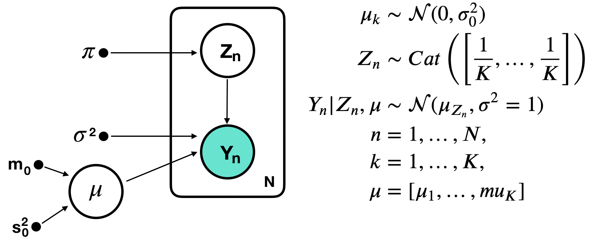
The hyperparameters of the models are \(\pi, \sigma^2, m_0, s^2_0\), which are constants that must be selected prior to inference. For example, to simplify our computations we selected \(\pi = [1/K, \ldots, 1/K]\), \(m_0 = 0\), \(\sigma=1\).

We make the mean field assumption – that our variational posterior factorizes completely:

\[q(Z, \mu| m, s^2, \phi) = \prod_{k=1}^K q(\mu_k|m_k, s_k^2) \prod_{n=1}^N q(Z_n|\phi_n).\]

Going deeper: Coordinate Ascent Variational Inference Updates for Bayesian GMM

In coordinate ascent variational inference, we update the variational distribution for each variable in turn. For the Bayesian GMM this means:

\[\begin{split}\begin{aligned} q(Z_n | \phi_n) &\propto \exp\left\{ \mathbb{E}_{\mu \sim q(\mu | m, s^2), Z_{-n} \sim q(Z_{-n} | \phi_{-n})}\left[\log p(Y_1, \ldots, Y_N, Z_1, \ldots, Z_N, \mu)\right]\right\}\\ q(\mu_k | m_k, s_k^2) &\propto \exp\left\{ \mathbb{E}_{Z \sim q(Z | \phi), q(\mu_{-k}|m_{-k}, s_{-k})}\left[\log p(Y_1, \ldots, Y_N, Z_1, \ldots, Z_N, \mu)\right]\right\} \end{aligned}\end{split}\]

where

\[\begin{split}\begin{aligned} q(\mu | m, s^2) &= \prod_{k=1}^K q(\mu_k|m_k, s_k^2),\\ q(\mu_{-k} | m_{-k}, s_{-k}^2) &= \prod_{j\neq k} q(\mu_j|m_j, s_j^2),\\ Z &= [Z_1\;\;\ldots\;\; Z_N],\\ q(Z |\phi) &= \prod_{n=1}^N q(Z_n|\phi_n),\\ Z_{-n} &= [Z_1\;\;\ldots\;\;Z_{n-1}\;\; Z_{n+1}\;\;\ldots\;\; Z_N],\\ q(Z_{-n} |\phi_{-n}) &= \prod_{m\neq n} q(Z_m|\phi_m). \end{aligned}\end{split}\]

Update rule for \(q(Z_n | \phi_n)\) To update \(q(Z_n | \phi_n)\), we rewrite \(exp\left\{ \mathbb{E}_{\mu \sim q(\mu | m, s^2), Z_{-n} \sim q(Z_{-n} | \phi_{-n})}\left[\log p(Y_1, \ldots, Y_N, Z_1, \ldots, Z_N, \mu)\right]\right\}\), dropping all terms that do not involve \(Z_n\) and \(\mu\):

\[\begin{split}\begin{aligned} q(Z_n | \phi_n) &\propto \exp\left\{ \mathbb{E}_{\mu \sim q(\mu | m, s^2), Z_{-n} \sim q(Z_{-n} | \phi_{-n})}\left[\log p(Y_1, \ldots, Y_N, Z_1, \ldots, Z_N, \mu)\right]\right\}\\ &= \exp\left\{ \mathbb{E}_{\mu \sim q(\mu | m, s^2), Z_{-n} \sim q(Z_{-n} | \phi_{-n})}\left[\log \left(\prod_{m=1}^N p(Y_m|\mu, Z_m) p(Z_m)\right)p(\mu)\right]\right\}\\ &= \exp\left\{ \mathbb{E}_{\mu \sim q(\mu | m, s^2), Z_{-n} \sim q(Z_{-n} | \phi_{-n})}\left[\log \left(\prod_{m=1}^N p(Y_m|\mu, Z_m) p(Z_m)\right)\right] + \log[p(\mu)]\right\}\\ &= \exp\left\{ \mathbb{E}_{\mu \sim q(\mu | m, s^2), Z_{-n} \sim q(Z_{-n} | \phi_{-n})}\left[\log \left(\prod_{m=1}^N p(Y_m|\mu, Z_m) p(Z_m)\right)\right]\right\} \exp\left\{ \log[p(\mu)]\right\}\\ &\propto \exp\left\{ \mathbb{E}_{\mu \sim q(\mu | m, s^2), Z_{-n} \sim q(Z_{-n} | \phi_{-n})}\left[\log \left(\prod_{m=1}^N p(Y_m|\mu, Z_m) p(Z_m)\right)\right]\right\}\quad\quad (\text{dropped priors on $\mu$})\\ &= \exp\left\{ \mathbb{E}_{\mu \sim q(\mu | m, s^2), Z_{-n} \sim q(Z_{-n} | \phi_{-n})}\left[\log \left(p(Y_n | \mu, Z_n) p(Z_n) \prod_{m\neq n} p(Y_m|\mu, Z_m) p(Z_m)\right)\right]\right\}\\ &= \exp\left\{ \mathbb{E}_{\mu \sim q(\mu | m, s^2), Z_{-n} \sim q(Z_{-n} | \phi_{-n})}\left[ \log p(Y_n | \mu, Z_n) + \log p(Z_n) + \sum_{m\neq n} \log \left( p(Y_m|\mu, Z_m) p(Z_m)\right) \right]\right\}\\ &= \exp\left\{ \mathbb{E}_{\mu \sim q(\mu | m, s^2)}\left[ \log p(Y_n | \mu, Z_n) + \log p(Z_n)\right] + \mathbb{E}_{\mu \sim q(\mu | m, s^2), Z_{-n} \sim q(Z_{-n} | \phi_{-n})}\left[\sum_{m\neq n} \log \left( p(Y_m|\mu, Z_m) p(Z_m)\right) \right]\right\}\\ &= \exp\left\{ \mathbb{E}_{\mu \sim q(\mu | m, s^2)}\left[ \log p(Y_n | \mu, Z_n) + \log p(Z_n)\right]\right\} \underbrace{\exp\left\{\mathbb{E}_{\mu \sim q(\mu | m, s^2), Z_{-n} \sim q(Z_{-n} | \phi_{-n})}\left[\sum_{m\neq n} \log \left( p(Y_m|\mu, Z_m) p(Z_m)\right) \right]\right\}}_{\text{constant with respect to $Z_n$}}\\ &\propto \exp\left\{ \mathbb{E}_{\mu \sim q(\mu | m, s^2)}\left[ \log p(Y_n | \mu, Z_n) + \log p(Z_n)\right]\right\} \quad\quad (\text{dropped all terms except for the $n$-th})\\ &= \exp\left\{ \mathbb{E}_{\mu \sim q(\mu | m, s^2)}\left[ \log p(Y_n | \mu, Z_n) \right]+ \mathbb{E}_{\mu \sim q(\mu | m, s^2)} \left[\log p(Z_n)\right]\right\}\\ &= \exp\left\{ \mathbb{E}_{\mu \sim q(\mu | m, s^2)}\left[ \log p(Y_n | \mu, Z_n) \right]+ \log p(Z_n)\right\}\\ &= \exp\left\{ \mathbb{E}_{\mu \sim q(\mu | m, s^2)}\left[ \log p(Y_n | \mu, Z_n) \right]+ \log \frac{1}{K}\right\}\\ &= \exp\left\{ \mathbb{E}_{\mu \sim q(\mu | m, s^2)}\left[ \log p(Y_n | \mu, Z_n) \right]\right\} \exp\left\{\log \frac{1}{K}\right\}\\ &\propto \exp\left\{ \mathbb{E}_{\mu \sim q(\mu | m, s^2)}\left[ \log p(Y_n | \mu, Z_n) \right]\right\}\quad\quad (\text{dropped the prior on $Z_n$})\\ \end{aligned}\end{split}\]

The likelihood \(p(Y_n | \mu, Z_n)\) is a normal distribution given the value of \(Z_n\), we can express this by treating each \(Z_n\) as an indicator variable – a \(K\)-dimensional binary vector with \(Z_{nk}=1\) if \(Y_n\) is in class \(k\) and 0 otherwise. Thus, we can write

\[\begin{split}\begin{aligned} \log p(Y_n | \mu, Z_n) &= \log \prod_{k=1}^K \mathcal{N}(Y_n; \mu_k, 1)^{Z_{nk}}\\ &= \sum_{k=1}^K Z_{nk} \log \mathcal{N}(Y_n; \mu_k, 1)\\ &= -\frac{1}{2}\sum_{k=1}^K Z_{nk} (Y_n - \mu_k)^2 + const\\ \end{aligned}\end{split}\]

Finally, we can write the update for \(q(Z_n | \phi_n)\) as follows, again dropping all terms not involving \(Z_n\) and \(\mu\):

\[\begin{split}\begin{aligned} q(Z_n | \phi_n) &\propto \exp\left\{ \mathbb{E}_{\mu \sim q(\mu | m, s^2)}\left[ -\frac{1}{2}\sum_{k=1}^K Z_{nk} (Y_n - \mu_k)^2 + const\right]\right\}\\ &= \exp\left\{ \mathbb{E}_{\mu \sim q(\mu | m, s^2)}\left[ -\frac{1}{2}\sum_{k=1}^K Z_{nk} (Y_n - \mu_k)^2\right]\right\} \exp\left\{\mathbb{E}_{\mu \sim q(\mu | m, s^2)} \left[const\right]\right\}\\ &\propto \exp\left\{ \mathbb{E}_{\mu \sim q(\mu | m, s^2)}\left[ -\frac{1}{2}\sum_{k=1}^K Z_{nk} (Y_n - \mu_k)^2\right]\right\}\\ &= \exp\left\{ -\frac{1}{2}\sum_{k=1}^K Z_{nk} \mathbb{E}_{\mu \sim q(\mu | m, s^2)}\left[Y^2_n - 2Y_n\mu_k + \mu_k^2\right]\right\}\\ &= \exp\left\{ -\frac{1}{2}\sum_{k=1}^K Z_{nk} \left(\mathbb{E}_{\mu \sim q(\mu | m, s^2)}\left[Y^2_n\right] - 2Y_n\mathbb{E}_{\mu \sim q(\mu | m, s^2)}\left[\mu_k\right] + \mathbb{E}_{\mu \sim q(\mu | m, s^2)}\left[\mu_k^2\right]\right)\right\}\\ &= \exp\left\{ -\frac{1}{2}\sum_{k=1}^K Z_{nk} \left(Y^2_n - 2Y_nm_k + (m_k + s_k^2)\right)\right\}\\ &= \exp\left\{ -\sum_{k=1}^K Z_{nk} Y^2_n +\sum_{k=1}^KZ_{nk}\left( Y_nm_k - \frac{(m_k + s_k^2)}{2}\right) \right\}\\ &= \exp\left\{ -\sum_{k=1}^K Z_{nk} Y^2_n\right\} \exp\left\{ \sum_{k=1}^KZ_{nk}\left( Y_nm_k - \frac{(m_k + s_k^2)}{2}\right) \right\}\\ &\propto \exp\left\{\sum_{k=1}^KZ_{nk}\left( Y_nm_k - \frac{(m_k + s_k^2)}{2}\right) \right\} \end{aligned}\end{split}\]

Since \(q(Z_n | \phi_n)\) is a categorical distribution, we can use the above to compute the \(k\)-th component as:

\[\begin{aligned} \phi_{nk}\propto \exp\left\{ Y_n m_k - \frac{(m_k + s_k^2)}{2} \right\} \end{aligned}\]

Update rule for \(q(\mu_k | m_k, s_k^2)\) To update \(q(\mu_k | m_k, s_k^2)\), we compute:

\[\begin{split}\begin{aligned} q(\mu_k | m_k, s_k^2) &\propto \exp\left\{ \mathbb{E}_{Z \sim q(Z | \phi), q(\mu_{-k}|m_{-k}, s_{-k})}\left[\log p(Y_1, \ldots, Y_N, \psi)\right]\right\}\\ &= \exp\left\{ \mathbb{E}_{Z \sim q(Z | \phi), q(\mu_{-k}|m_{-k}, s_{-k})}\left[\log \left(\prod_{n=1}^N p(Y_n|\mu, Z_n) p(Z_n)\right) p(\mu)\right] \right\}\\ &= \exp\left\{ \mathbb{E}_{Z \sim q(Z | \phi), q(\mu_{-k}|m_{-k}, s_{-k})}\left[\log \left(\prod_{n=1}^N p(Y_n|\mu, Z_n) \right) p(\mu)\right] + \log \prod_{n=1}^N p(Z_n) \right\}\\ &= \exp\left\{ \mathbb{E}_{Z \sim q(Z | \phi), q(\mu_{-k}|m_{-k}, s_{-k})}\left[\log \left(\left(\prod_{n=1}^N p(Y_n|\mu, Z_n) \right)p(\mu)\right) \right] \right\} \exp\left\{\log \prod_{m=1}^Mp(Z_m) \right\}\\ &\propto \exp\left\{ \mathbb{E}_{Z \sim q(Z | \phi), q(\mu_{-k}|m_{-k}, s_{-k})}\left[\log \left(\prod_{k=1}^K \prod_{n=1}^N p(Y_n|\mu_k, Z_n) \prod_{k=1}^K p(\mu_k)\right) \right] \right\}\\ &= \exp\left\{ \mathbb{E}_{Z \sim q(Z | \phi), q(\mu_{-k}|m_{-k}, s_{-k})}\left[\log \left(\prod_{n=1}^N p(Y_n|\mu_k, Z_n) p(\mu_k) \left(\prod_{j\neq k} \prod_{n=1}^N p(Y_n|\mu_j, Z_n) \prod_{j\neq k} p(\mu_j)\right) \right)\right] \right\}\\ &= \exp\left\{ \mathbb{E}_{Z \sim q(Z | \phi), q(\mu_{-k}|m_{-k}, s_{-k})}\left[\log \left(\prod_{n=1}^N p(Y_n|\mu_k, Z_n) p(\mu_k)\right) + \log \left(\prod_{j\neq k} \prod_{n=1}^N p(Y_n|\mu_j, Z_n) \prod_{j\neq k} p(\mu_j)\right)\right] \right\}\\ &= \exp\left\{ \mathbb{E}_{Z \sim q(Z | \phi), q(\mu_{-k}|m_{-k}, s_{-k})}\left[\log \left(\prod_{n=1}^N p(Y_n|\mu_k, Z_n) p(\mu_k)\right)\right] + \mathbb{E}_{Z \sim q(Z | \phi), q(\mu_{-k}|m_{-k}, s_{-k})}\left[\log \left(\prod_{j\neq k} \prod_{n=1}^N p(Y_n|\mu_j, Z_n) \prod_{j\neq k} p(\mu_j)\right)\right] \right\}\\ &= \exp\left\{ \mathbb{E}_{Z \sim q(Z | \phi)}\left[\log \left(\prod_{n=1}^N p(Y_n|\mu_k, Z_n) p(\mu_k)\right)\right] \right\} \exp\left\{ \mathbb{E}_{Z \sim q(Z | \phi), q(\mu_{-k}|m_{-k}, s_{-k})}\left[\log \left(\prod_{j\neq k} \prod_{n=1}^N p(Y_n|\mu_j, Z_n) \prod_{j\neq k} p(\mu_j)\right)\right] \right\}\\ &\propto \exp\left\{ \mathbb{E}_{Z \sim q(Z | \phi)}\left[\log \left(\prod_{n=1}^N p(Y_n|\mu_k, Z_n) p(\mu_k)\right)\right] \right\} &=\exp\left\{ \mathbb{E}_{Z \sim q(Z | \phi)}\left[\sum_{n=1}^N \log p(Y_n|\mu_k, Z_n) + \log p(\mu_k)\right] \right\}\\ &= \exp\left\{ \mathbb{E}_{Z \sim q(Z | \phi)}\left[\sum_{n=1}^N \sum_{j=1}^K Z_{nj}\log \mathcal{N}(Y_n; \mu_j, 1) + \log \mathcal{N}(\mu_k; 0, s^2_0)\right] \right\}\\ &= \exp\left\{ \sum_{n=1}^N \sum_{j=1}^K \mathbb{E}_{Z \sim q(Z | \phi)}\left[Z_{nj}\right]\log \mathcal{N}(Y_n; \mu_j, 1) + \log \mathcal{N}(\mu_k; 0, s^2_0) \right\}\\ &= \exp\left\{ \sum_{n=1}^N \sum_{j=1}^K \phi_{nj}\log \mathcal{N}(Y_n; \mu_j, 1) + \log \mathcal{N}(\mu_k; 0, s^2_0) \right\}\\ &= \exp\left\{ \sum_{n=1}^N \phi_{nk}\log \mathcal{N}(Y_n; \mu_k, 1) + \log \mathcal{N}(\mu_k; 0, s^2_0) + \sum_{n=1}^N \sum_{j\neq k} \phi_{nj}\log \mathcal{N}(Y_n; \mu_j, 1) \right\}\\ &= \exp\left\{ \sum_{n=1}^N \phi_{nk}\log \mathcal{N}(Y_n; \mu_k, 1) + \log \mathcal{N}(\mu_k; 0, s^2_0)\right\} \exp\left\{\sum_{n=1}^N \sum_{j\neq k} \phi_{nj}\log \mathcal{N}(Y_n; \mu_j, 1) \right\}\\ &\propto \exp\left\{ \sum_{n=1}^N \phi_{nk}\log \mathcal{N}(Y_n; \mu_k, 1) + \log \mathcal{N}(\mu_k; 0, s^2_0)\right\}\\ &= \exp\left\{ \sum_{n=1}^N \phi_{nk} \frac{(y_n-\mu_k)^2}{2} - \frac{\mu_k^2}{2\sigma_0^2} + const\right\}\\ &= \exp\left\{ \sum_{n=1}^N \phi_{nk} \frac{(y_n-\mu_k)^2}{2} - \frac{\mu_k^2}{2\sigma_0^2}\right\}\exp\left\{const\right\}\\ &\propto \exp\left\{ \sum_{n=1}^N \phi_{nk} \frac{(y_n-\mu_k)^2}{2} - \frac{\mu_k^2}{2\sigma_0^2}\right\}\\ &= \exp\left\{ \left(\sum_{n=1}^N \phi_{nk} y_n\right)\mu_k - \frac{1}{2}\left(\sum_{n=1}^N \phi_{nk} + \frac{1}{\sigma_0^2}\right)\mu^2_k + const\right\}\\ &= \exp\left\{ \left(\sum_{n=1}^N \phi_{nk} y_n\right)\mu_k - \frac{1}{2}\left(\sum_{n=1}^N \phi_{nk} + \frac{1}{\sigma_0^2}\right)\mu^2_k\right\} \exp\left\{ const\right\}\\ &\propto \exp\left\{ \underbrace{\left(\sum_{n=1}^N \phi_{nk} y_n\right)}_{A}\mu_k - \underbrace{\frac{1}{2}\left(\sum_{n=1}^N \phi_{nk} + \frac{1}{\sigma_0^2}\right)}_{B}\mu^2_k\right\} \\ &= \exp\left\{ - (B\mu_k^2 - A\mu_k)\right\}\\ &= \exp\left\{ - B\left(\mu_k^2 - \frac{A}{B}\mu_k + \left( \frac{A}{2B}\right)^2 - \left( \frac{A}{2B}\right)^2 \right)\right\}\\ &= \exp\left\{ - B\left(\mu_k^2 - \frac{A}{2B}\right)^2 - B\left( \frac{A}{2B}\right)^2 \right\}\\ &= \exp\left\{ - B\left(\mu_k^2 - \frac{A}{2B}\right)^2\right\} \exp\left\{- B\left( \frac{A}{2B}\right)^2 \right\}\\ &\propto \exp\left\{ - B\left(\mu_k^2 - \frac{A}{2B}\right)^2\right\} \end{aligned}\end{split}\]

Thus, we see that \(q(\mu_k | m_k, s_k^2) \propto \exp\left\{ - B\left(\mu_k^2 - \frac{A}{2B}\right)^2\right\} \) is a Gaussian with mean

\[m_k = \frac{A}{2B} = \frac{\sum_{n=1}^N \phi_{nk} y_n}{\sum_{n=1}^N \phi_{nk} + \frac{1}{\sigma_0^2}},\]

and variance

\[s^2_k = \frac{1}{2B} = \frac{1}{\sum_{n=1}^N \phi_{nk} + \frac{1}{\sigma_0^2}}.\]

Implementation of CAVI for Bayesian GMM

Show code cell content

Hide code cell content

#Generate data
N = 2000
pis = [1./3, 1./3, 1./3]
mus = [6, 10, 14]
sigmas = [1., 1., 1.]
K = 3
zs = np.random.choice(np.arange(K), size=N, p=pis)
y = np.array([np.random.normal(mus[z], sigmas[z]**0.5, 1)[0] for z in zs])

#defining the bayesian model
sigma_sq = 1.**2
s_sq_0 = 1.

#initialization for CAVI
m_init = np.array([2, 4, 5])
s_sq_init = np.array([1., 1., 1.])

#implement coordinate ascent VI
m_current = m_init
s_sq_current = s_sq_init

total_iter = 10000
threshold = 1e-10
delta_m = 1.
delta_s = 1.
i = 0

#implementation of the ELBO
def elbo(m, s_sq, phi):
    summand_1 = (np.log(s_sq) - m / s_sq_0).sum()
    summand_2 = ((-0.5 * np.add.outer(y**2, s_sq + m**2) + np.outer(y, m) - np.log(phi)) * phi).sum()
    return summand_1 + summand_2

ELBOs = []
while i < total_iter and delta_m > threshold and delta_s > threshold:
    #update q(Z_n)
    exponent = np.outer(y, m_current) + -(0.5 * m_current**2 + 0.5 * s_sq_current)[np.newaxis, :]
    phi_unnormalized = np.exp(exponent)
    phi = phi_unnormalized / phi_unnormalized.sum(1)[:, np.newaxis]
    #update mu
    m_new = (phi * y[:, np.newaxis]).sum(0) * (1. / s_sq_0 + phi.sum(0))**(-1)
    #update s squared 
    s_sq_new = (1. / s_sq_0 + phi.sum(0))**(-1)
    
    #compute ELBO
    ELBOs.append(elbo(m_new, s_sq_new, phi))
    
    #compute variational parameter change
    delta_m = np.linalg.norm(m_new - m_current)
    delta_s = np.linalg.norm(s_sq_new - s_sq_current)
    
    m_current = m_new
    s_sq_current = s_sq_new
    
    i += 1
    
#sample from posterior predictive    
def posterior_predictive_sampling(means, variances, S):
    posterior_predictive_samples = []
    for mean, variance in zip(means, variances):
        posterior_samples = np.random.normal(mean, variance**2, size=S)
        posterior_predictive_samples += [np.random.normal(sample, sigma_sq**2, 1)[0] for sample in posterior_samples]
    return np.array(posterior_predictive_samples)
    
x = np.linspace(y.min(), y.max(), 1000)

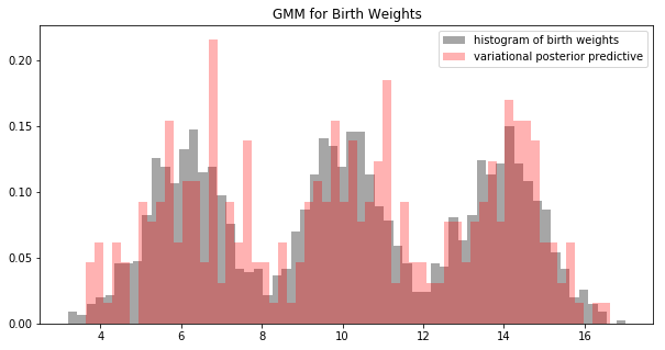
fig, ax = plt.subplots(1, 1, figsize=(10, 5))
ax.hist(y, bins=60, density=True, color='gray', alpha=0.7, label='histogram of birth weights')
posterior_predictive_samples = posterior_predictive_sampling(m_current, s_sq_current, 100)
ax.hist(posterior_predictive_samples, bins=60, density=True, color='red', alpha=0.3, label='variational posterior predictive')
ax.set_title('GMM for Birth Weights')
ax.legend(loc='best')
plt.show()

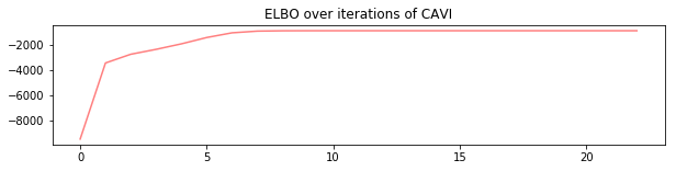
Sanity Check: ELBO During Training

Remember that plotting the posterior predictive against actual data is not always an option (e.g. high-dimensional data).

A sanity check for that your CAVI algorithm has been implemented correctly is to plot the ELBO (or alternatively, the observed data log-likelihood) over the iterations of the algorithm:

\[ ELBO(\phi, m, s^2) = \mathbb{E}_{Z, \mu\sim q(Z, \mu | \phi, m, s^2)} \left[\log \left( \frac{p(Y_1, \ldots, Y_N, Z_1, \ldots, Z_N, \mu)}{q(Z, \mu | \phi, m, s^2)}\right) \right] \]

fig, ax = plt.subplots(1, 1, figsize=(10, 2))
ax.plot(range(len(ELBOs)), ELBOs, color='red', alpha=0.5)
ax.set_title('ELBO over iterations of CAVI')
plt.show()

12.2. Exercises

These problems were originally assigned as homework. Data files are in the book’s data/ folder. Worked solutions, where available, are collapsed beneath the questions they answer; try each problem before expanding them.

Problem Set: Understanding EM and Variational Inference

Show code cell content

Hide code cell content

### Import basic libraries
import numpy as np
import pandas as pd
import sklearn as sk
from sklearn.linear_model import LinearRegression
import matplotlib.pyplot as plt
%matplotlib inline

Show code cell content

Hide code cell content

# data_df is the dataframe of your data
# estimates_df is a numpy array of cancer rate estimates, one for each county
def scatter_plot_cancer_rates(data_df, estimates=None):
    ax = data_df.plot(kind='scatter', x="pop",y="pct_mortality", alpha=0.0001, color="grey")
    bot_kcancer_counties = data_df.sort_values(by='pct_mortality',ascending=True)[:300]
    top_kcancer_counties = data_df.sort_values(by='pct_mortality',ascending=False)[:300]
    top_kcancer_counties.plot(kind='scatter',x="pop",y="pct_mortality",alpha=0.0001, color="blue", ax=ax, logx=True)
    bot_kcancer_counties.plot(kind='scatter',x="pop",y="pct_mortality",alpha=0.0001, color="red", ax=ax, logx=True)
    if estimates is not None:
        ax.plot(data_df['pop'], 5 * estimates, '.', alpha=0.2, color="green")
    ax.set_ylim([-0.0001, 0.0003])

In this problem, we will draw concrete connections between EM and variational inference by applying both methods to a certain class of latent variable models. You’ll need to refer to the derivation of EM in Chapter 11 and the derivation of the variational inference objective earlier in this chapter. This is an essay question that requires you to engage with complex derivations at a productive but still high level. No implementation is required.

Non-Bayesian Latent Variable Model

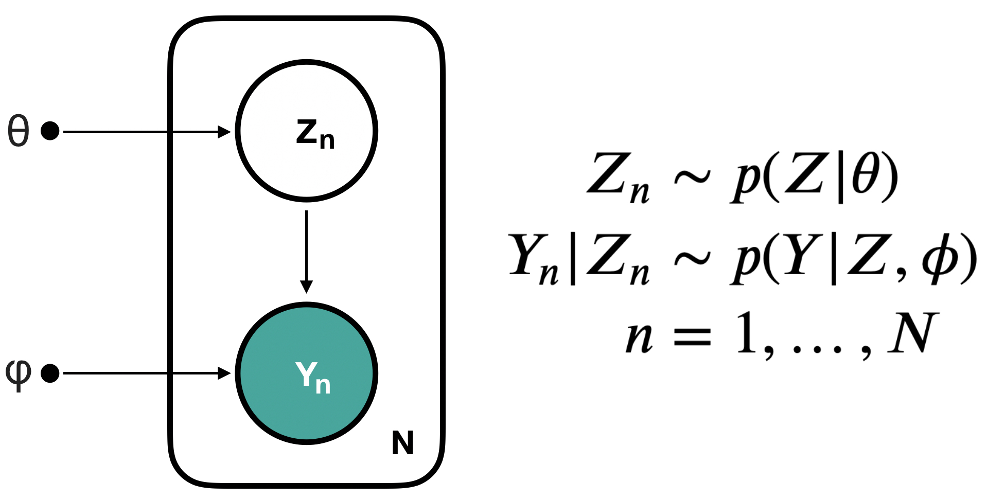
Recall the class of latent variable models we studied in Chapter 11:

Bayesian Latent Variable Model

A Bayesian version of the same class of models involve adding priors for the model parameters:

1. (Comparing ELBOs) For the above type of Bayesian latent variable model, write down the ELBO for variational inference with a mean field variational family. Compare the variational inference ELBO for the Bayesian model to the expectation maximization ELBO for the non-Bayesian model. What are the differences and similarities between these two ELBOs?

   In both EM and variational inference we optimize the ELBO. Compare the update steps in EM to the update steps in Coordinate Ascent Variational Inference, draw a concrete analogy between them.

   Hint: To make both ELBO’s comparable, make sure that both are in terms of \(z, y, \theta, \phi\).
   
   

2. (Comparing ELBOs and KL-divergences) Recall that the original objective of variational inference is to minimize a KL-divergence, we rewrote the objective to be that of maximizing the ELBO. Why is directly minimizing the KL-divergence in the original objective difficult (be specific about wherein the difficulty lies)?

   In the derivation of the E-step of EM, we reframed an maximization of the ELBO problem as a minimization of a KL-divergence problem. In this case, why was the KL-divergence easier to minimize and the ELBO harder to maximize (use the instantiation of the E-step for Gaussian Mixture Models in Chapter 11 to help support your answer)?

   Earlier in this chapter, we introduced a way to maximize the variational inference ELBO – through coordinate ascent. In the derivation of the updates for coordinate ascent, there is a place where we reframed an maximization of the ELBO problem as an equivalent minimization of a KL-divergence problem. Write down the exact form of this equivalence (the two expressions are separated in the derivation by a bunch of lines, you’ll need to identify both parts that you need). In this case, why was the KL-divergence easier to minimize and the ELBO harder to maximization (use the instantiation of the update for Gaussian Mixture Models earlier in this chapter to help support your answer)?

   Based on this analysis, can you draw some general conclusions about when we’d prefer to minimize the KL-divergence versus when we’d prefer to maximize the ELBO?
   
   

3. (The Mean Field Assumption and Coordinate Ascent) Describe exactly when and how the mean field assumption is used in the derivation of the coordinate ascent updates.
   
   

4. (Generalizability of CAVI) Summarize what kind of derivations/math is needed in order instantiate Coordinate Ascent Variational Inference (CAVI) for a given new model (look at what we did for Gaussian Mixture Models earlier in this chapter and predict what you’d need to do for a new model). Based on this, discuss the potential draw backs of using CAVI for Bayesian inference in general. What do these draw backs imply about the practicality of variational inference as an inference method?
   
   

5. (Generalizability of EM) Summarize what kind of derivations/math is needed in order instantiate Expectation Maximization (EM) for a given new model (look at what we did for Gaussian Mixture Models in Chapter 11 and predict what you’d need to do for a new model). Based on this, discuss the potential draw backs of using EM for MLE inference in general. What do these draw backs imply about the practicality of EM as an inference method?

Solution: Question 1

Recall that the EM ELBO for this type of latent variable model is

\[ ELBO^{\text{EM}}(\theta, \phi, q(z)) = \mathbb{E}_{z\sim q(z)}\left[\log\left(\frac{p(y, z|\theta, \phi)}{q(z)}\right)\right] \]

whereas the variational inference ELBO for the Bayesian version of this type of latent variable model is

\[ ELBO^{\text{VI}}(q(\theta|\lambda_2), q(\phi|\lambda_1), q(z|\lambda_3)) = \mathbb{E}_{z, \phi, \theta \sim q(z, \phi, \theta |\lambda_1, \lambda_2, \lambda_3)} \left[\log\left(\frac{p(y, z, \theta, \phi|a, b)}{q(z, \phi, \theta |\lambda_1, \lambda_2, \lambda_3)}\right)\right] \]

The similarity between these two ELBO is that they are both expected log ratios between a joint distribution \(p\) and an auxiliary or approximating distribution \(q\). In the case of EM, we are measuring the expected (under \(q\)) log ratio between the auxiliary distribution \(q(z)\) and the joint \(p(y, z|\theta, \phi)\); in the case of variational inference we are measuring the expected log ratio between the variational distribution \(q(z, \phi, \theta |\lambda_1, \lambda_2, \lambda_3)\) and the joint \(p(y, z, \theta, \phi|a, b)\).

The major difference is how the parameters \(\theta\) and \(\phi\) are treated in the two ELBOs. For EM, we treat \(\theta\) and \(\phi\) as point masses, in variational inference we treat them as random variables with distributions. In EM, we optimize the ELBO with respect to \(\theta\) and \(\phi\) as point-masses where as in variational inference we optimize the distribution of \(\theta\) and \(\phi\). Note that the random variable \(z\) plays the same role in both ELBOs.

For those interested in a deeper connection: We can actually prove that EM is a special case of variational inference, by:

1. imposing flat priors for \(\theta\) and \(\phi\)

2. performing variational inference on this model with delta distributions for \(q(\theta)\) and \(q(\phi)\)

You’ll derive the same ELBO for variational inference as that for the EM estimation of the MLE of \(\theta, \phi\).

Not covered here: a comparison of the EM update steps with the CAVI update steps.

Solution: Question 2

Variational Objective In variational inference, we are interested in finding a tractable distribution \(q\) that best approximates a complex distribution \(p\). For the latent variable model considered in this problem, the variational objective is

\[ \underset{\lambda}{\min} D_{\text{KL}}[q(z, \phi, \theta |\lambda_1, \lambda_2, \lambda_3) \| p(z, \theta, \phi|y, a, b)] = \underset{\lambda}{\min} \mathbb{E}_{z, \phi, \theta \sim q(z, \phi, \theta |\lambda_1, \lambda_2, \lambda_3)} \left[\log \left( \frac{q(z, \phi, \theta |\lambda_1, \lambda_2, \lambda_3)}{p(z, \theta, \phi|y, a, b)}\right) \right] \]

Recall that the posterior \(p(z, \theta, \phi|y, a, b)\) is actually equal to

\[ p(z, \theta, \phi|y, a, b) = \frac{p(y, z, \theta, \phi| a, b)}{p(y | a, b)} = \frac{p(y, z, \theta, \phi| a, b)}{\int p(y, z, \theta, \phi| a, b)\, dz\, d\theta\, d\phi} \]

So when we substitute this into the expression of the KL-divergence, we can write:

\[\begin{split}\begin{aligned} D_{\text{KL}}[q(z, \phi, \theta |\lambda_1, \lambda_2, \lambda_3) \| p(z, \theta, \phi|y, a, b)] &= \mathbb{E}_{z, \phi, \theta \sim q(z, \phi, \theta |\lambda_1, \lambda_2, \lambda_3)} \left[\log \left( \frac{q(z, \phi, \theta |\lambda_1, \lambda_2, \lambda_3)}{p(z, \theta, \phi|y, a, b)}\right) \right]\\ =& \mathbb{E}_{z, \phi, \theta \sim q(z, \phi, \theta |\lambda_1, \lambda_2, \lambda_3)} \left[\log \left( \frac{q(z, \phi, \theta |\lambda_1, \lambda_2, \lambda_3)p(y | a, b)}{p(y, z, \theta, \phi| a, b)}\right) \right]\\ =& \mathbb{E}_{z, \phi, \theta \sim q(z, \phi, \theta |\lambda_1, \lambda_2, \lambda_3)} \left[\log q(z, \phi, \theta |\lambda_1, \lambda_2, \lambda_3) + \log p(y | a, b) - \log p(y, z, \theta, \phi| a, b) \right]\\ =& \mathbb{E}_{z, \phi, \theta \sim q(z, \phi, \theta |\lambda_1, \lambda_2, \lambda_3)} \left[\log q(z, \phi, \theta |\lambda_1, \lambda_2, \lambda_3)\right] \\ &+ \mathbb{E}_{z, \phi, \theta \sim q(z, \phi, \theta |\lambda_1, \lambda_2, \lambda_3)}\left[\log p(y | a, b)\right] \\ &- \mathbb{E}_{z, \phi, \theta \sim q(z, \phi, \theta |\lambda_1, \lambda_2, \lambda_3)}\left[\log p(y, z, \theta, \phi| a, b) \right]\\ \end{aligned}\end{split}\]

Note that the second term in the KL-divergence above is hard to compute:

\[ \mathbb{E}_{z, \phi, \theta \sim q(z, \phi, \theta |\lambda_1, \lambda_2, \lambda_3)}\left[\log p(y | a, b)\right] = \mathbb{E}_{z, \phi, \theta \sim q(z, \phi, \theta |\lambda_1, \lambda_2, \lambda_3)}\left[\log \int p(y, z, \theta, \phi| a, b)\, dz\, d\theta\, d\phi\right] \]

Now, when we work with the ELBO for variational inference, we have that

\[\begin{split}\begin{aligned} ELBO^{\text{VI}}(q(\theta|\lambda_2), q(\phi|\lambda_1), q(z|\lambda_3)) &= \mathbb{E}_{z, \phi, \theta \sim q(z, \phi, \theta |\lambda_1, \lambda_2, \lambda_3)} \left[\log\left(\frac{p(y, z, \theta, \phi|a, b)}{q(z, \phi, \theta |\lambda_1, \lambda_2, \lambda_3)}\right)\right]\\ &= \mathbb{E}_{z, \phi, \theta \sim q(z, \phi, \theta |\lambda_1, \lambda_2, \lambda_3)}\left[\log p(y, z, \theta, \phi| a, b) \right] - \mathbb{E}_{z, \phi, \theta \sim q(z, \phi, \theta |\lambda_1, \lambda_2, \lambda_3)} \left[\log q(z, \phi, \theta |\lambda_1, \lambda_2, \lambda_3)\right] \end{aligned}\end{split}\]

That is, the problematic term \(\mathbb{E}_{z, \phi, \theta \sim q(z, \phi, \theta |\lambda_1, \lambda_2, \lambda_3)}\left[\log p(y | a, b)\right]\) is gone!

This is why we say that the ELBO is easier to work with than the KL for variational inference.

The E-step in EM In the E-step of EM we had to compute

\[ \underset{q}{\max} ELBO^{\text{EM}}(\theta^*, \phi^*, q(z)) = \underset{q}{\max} \mathbb{E}_{z\sim q(z)}\left[\log\left(\frac{p(y, z|\theta^*, \phi^*)}{q(z)}\right)\right] \]

where \(\theta^*, \phi^*\) are the optimal values we found in the \(M\)-step.

In order to optimize this ELBO, we needed to take the “gradient” with respect to \(q\)

\[ \nabla_q \mathbb{E}_{z\sim q(z)}\left[\log\left(\frac{p(y, z|\theta^*, \phi^*)}{q(z)}\right)\right] \]

But since the expectation is also with respect to \(q\), this gradient is hard to compute!

Converting the problem of maximizing the ELBO into one of minimizing a KL-divergence

\[ \underset{q}{\max} ELBO^{\text{EM}}(\theta^*, \phi^*, q(z)) \equiv \underset{q}{\min} D_{\text{KL}}[q(z)\| p(z|y, \theta, \phi) ] \]

meant that we can solve the optimization problem immediately – by setting \(q(z)\) equal to \(p(z|y, \theta, \phi)\). In the case, of the Gaussian Mixture Model, the posterior \(p(z|y, \theta, \phi)\) was not difficult to compute. Since the latent variable \(z\) is a categorical variable, we could compute the probability of each class membership \(z=k\) independently. Each computation was very tractable.

The Derivation of the Update for CAVI Let \(\phi = [\phi_1,\ldots, \phi_I]\) be the set of parameters and latent variables for which we want to infer a posterior \(p(\phi | y_1, \ldots y_N)\). We approximate this posterior with a mean field variational family:

\[ q(\phi | \lambda) = \prod_{i=1}^I q(\phi_i | \lambda_i) \]

In CAVI, we update the variational distribution for each \(\phi_j\), conditioned on the other \(\phi\)’s by the rule:

\[ q(\phi_i | \lambda_i) \propto \exp\left\{ \mathbb{E}_{\psi_{-i} \sim q(\phi_{-i} | \lambda^{\text{new}}_{1}, \ldots, \lambda^{\text{new}}_{i-1}, \lambda^{\text{old}}_{i+1}, \ldots, \lambda^{\text{old}}_{I})}\left[\log p(Y_1, \ldots, Y_N, \psi)\right]\right\} \]

where \(\psi_{-i} = [\psi_1\; \ldots\; \psi_{i-1}\; \psi_{i+1}\; \ldots\; \psi_{I}]\).

To prove that this is the update that would maximize the ELBO for the coordinate \(i\), we transformed the problem of maximizing the variational inference ELBO with respect to \(q(\phi_i | \lambda_i)\) into a problem of minimizing a KL-divergence between \(q(\phi_i | \lambda_i)\) and some other distribution:

\[\begin{split}\begin{aligned} \underset{\lambda_i}{\max} ELBO(\lambda) &= \underset{\lambda_i}{\max} \int_{\Psi} \left[ \log \left(\frac{p(Y_1, \ldots, Y_N, \psi)}{q(\psi|\lambda)} \right)\right]q(\psi|\lambda) d\psi\\ &= \underset{\lambda_i}{\max} \mathbb{E}_{\psi_i \sim q(\psi_i|\lambda_i)}\left[ \log \left(\frac{\exp\left\{\mathbb{E}_{\psi_{-i} \sim q(\psi_{-i}|\lambda_{-i})} \left[\log \left(p(Y_1, \ldots, Y_N, \psi_i | \psi_{-i}) \right)\right]\right\} } {q(\psi_{i}|\lambda_{i})} \right)\right]\\ &\equiv \underset{\lambda_i}{\min} -\mathbb{E}_{\psi_i \sim q(\psi_i|\lambda_i)}\left[ \log \left(\frac{\exp\left\{\mathbb{E}_{\psi_{-i} \sim q(\psi_{-i}|\lambda_{-i})} \left[\log \left(p(Y_1, \ldots, Y_N, \psi_i | \psi_{-i}) \right)\right]\right\} } {q(\psi_{i}|\lambda_{i})} \right)\right]\\ &= \underset{\lambda_i}{\min} \underbrace{\mathbb{E}_{\psi_i \sim q(\psi_i|\lambda_i)}\left[ \log \left(\frac{ q(\psi_{i}|\lambda_{i}) } {\exp\left\{\mathbb{E}_{\psi_{-i} \sim q(\psi_{-i}|\lambda_{-i})} \left[\log \left(p(Y_1, \ldots, Y_N, \psi_i | \psi_{-i}) \right)\right]\right\} } \right)\right]}_{\text{looks like a KL except the denominator is not a distribution}}\quad (\text{using the properties of log})\\ &= \underset{\lambda_i}{\min} \mathbb{E}_{\psi_i \sim q(\psi_i|\lambda_i)}\left[ \log \left(\frac{ \mathcal{Z} q(\psi_{i}|\lambda_{i}) } {\mathcal{Z}\exp\left\{\mathbb{E}_{\psi_{-i} \sim q(\psi_{-i}|\lambda_{-i})} \left[\log \left(p(Y_1, \ldots, Y_N, \psi_i | \psi_{-i}) \right)\right]\right\} } \right)\right],\quad (\mathcal{Z} \text{ normalizes the denominator})\\ &= \underset{\lambda_i}{\min} \mathbb{E}_{\psi_i \sim q(\psi_i|\lambda_i)}\left[ \log \left(\frac{ q(\psi_{i}|\lambda_{i}) } {\mathcal{Z}\exp\left\{\mathbb{E}_{\psi_{-i} \sim q(\psi_{-i}|\lambda_{-i})} \left[\log \left(p(Y_1, \ldots, Y_N, \psi_i | \psi_{-i}) \right)\right]\right\} } \right)\right] +\log(\mathcal{Z})\\ &\equiv \underset{\lambda_i}{\min}D_{\text{KL}} \left[ q(\psi_{i}|\lambda_{i})\| \mathcal{Z}\exp\left\{\mathbb{E}_{\psi_{-i} \sim q(\psi_{-i}|\lambda_{-i})} \left[\log \left(p(Y_1, \ldots, Y_N, \psi_i | \psi_{-i}) \right)\right]\right\}\right]. \end{aligned}\end{split}\]

The optimization problem involving the KL-divergence was again easy to solve! We just set \(q(\psi_{i}|\lambda_{i})\) equal to \(\mathcal{Z}\exp\left\{\mathbb{E}_{\psi_{-i} \sim q(\psi_{-i}|\lambda_{-i})} \left[\log \left(p(Y_1, \ldots, Y_N, \psi_i | \psi_{-i}) \right)\right]\right\}\).

So why do we prefer to evaluate this complicated expression \(q(\psi_{i}|\lambda_{i})\) equal to \(\mathcal{Z}\exp\left\{\mathbb{E}_{\psi_{-i} \sim q(\psi_{-i}|\lambda_{-i})} \left[\log \left(p(Y_1, \ldots, Y_N, \psi_i | \psi_{-i}) \right)\right]\right\}\)?

For one, maximizing the ELBO requires taking a gradient with respect to a variable that the expectation depends on: \(\nabla_{\lambda_i} \mathbb{E}_{\psi_i \sim q(\psi_i|\lambda_i)}\left[ \ldots \right]\). This, again, is a hard problem to solve.

Secondly, the expectation \(\mathbb{E}_{\psi_{-i} \sim q(\psi_{-i}|\lambda_{-i})} \left[\log \left(p(Y_1, \ldots, Y_N, \psi_i | \psi_{-i}) \right)\right]\) is not intractable to compute for nice models like Gaussian Mixture Models. Due to the way that these models factorize – in each update, we end up working with one term involving \(\phi_i\), since the other terms involving \(\phi_{-i}\) become constants after taking the expectation \(\mathbb{E}_{\psi_{-i} \sim q(\psi_{-i}|\lambda_{-i})}\).

When to Work with the ELBO and When to Work with a KL? The general rule of thumb is intuitive: if the posterior \(p(A|B)\) is known and tractable then minimizing the KL-divergence \(D_{\text{KL}}[q(A)\|p(A|B)]\) by setting \(q\) equal to \(p\) is preferred. If \(p(A|B)\) is not known or tractable, but the joint \(p(A, B)\) is tractable then it’s preferable to work with the ELBO \(\mathbb{E}_{q(A)}\left[\log \frac{p(A, B)}{q(A)}\right]\).

Solution: Question 3

The mean field assumption allows us to rewrite the expectation in the ELBO over all \(\psi_i\)’s jointly as iterated expectation:

\[ ELBO(\lambda) = \mathbb{E}_{\psi \sim q(\psi|\lambda)}[\ldots] = \mathbb{E}_{\psi_i \sim q(\psi_i|\lambda_i)}\left[\mathbb{E}_{\psi_{-i} \sim q(\psi_{-i}|\lambda_{-i})}[\ldots] \right] \]

When we modeled \(\psi\)’s as independent under the variational distribution \(q\), we were able to apply Fubini’s theorem to the integral that defined \(\mathbb{E}_{\psi \sim q(\psi|\lambda)}\) – i.e. we turned a integral over multiple variables into an iterated integral.

Solution: Question 4

Given a model with a posterior over variable \(\psi_1, \ldots, \psi_I\), we’d need to set \(q(\psi_{i}|\lambda_{i})\) equal to \(\mathcal{Z}\exp\left\{\mathbb{E}_{\psi_{-i} \sim q(\psi_{-i}|\lambda_{-i})} \left[\log \left(p(Y_1, \ldots, Y_N, \psi_i | \psi_{-i}) \right)\right]\right\}\) for every \(i\), in order to iteratively maximize the ELBO.

For example, in the Bayesian Gaussian mixture case, we had to derive the update for \(q(z|\phi)\) and \(q(\mu_k|m_k, s_k^2)\) for each component \(k\) in the mixture. Each derivation required an immense amount of algebra. Further more each derivation was different in nature – for \(q(z|\phi)\) we used the fact that \(z\) is a categorical variable to compute the probability of \(z=k\) individually, for \(q(\mu_k|m_k, s_k^2)\) we had to complete the square to make the expression

\[\mathcal{Z}\exp\left\{\mathbb{E}_{\psi_{-i} \sim q(\psi_{-i}|\lambda_{-i})} \left[\log \left(p(Y_1, \ldots, Y_N, \psi_i | \psi_{-i}) \right)\right]\right\}\]

look like the pdf of a Gaussian.

This is a process that is highly specialized to the specific model we’re given.

One can imagine that if you wanted to implement CAVI for a new model, you’d have to do the entire set of derivations from scratch!

This prevents us from applying variational inference easily to new models and may prevent us from applying variational inference entirely if we are unable to complete these derivations. In order to make variational inference broadly applicable to a large class of Bayesian models we need an automatic and efficient way of

1. computing the gradient of the ELBO

2. finding the stationary points of this gradient

12.3. Further Reading

Variational Inference

• (Introductory) Coordinate Ascent Mean-field Variational Inference (Univariate Gaussian Example)

• (In-Depth) Variational Inference: A Review for Statisticians

• (Introductory) Kullback-Leibler divergence

• (Advanced) Shannon Entropy and Kullback-Leibler Divergence