16. Stochastic Gradient Descent and Simulated Annealing#
This chapter is adapted from AM207 (Harvard, Fall 2021). Watch the recorded lecture.
In this chapter
Generalized Linear Models
Stochastic Gradient Descent
Non-Convex Optimization
Simulated Annealing
16.1. Generalized Linear Models#
A New Model: Logistic Regression#
A logistic regression model is just a Bernoulli model \(Y^{(n)} \sim Ber(\theta_n)\) model, where \(\theta^{(n)}\) depends on a set of covariates \(\theta^{(n)} =\mathrm{sigm}(f(\mathbf{X}; \mathbf{w}))\). For now, we assume that \(f(\mathbf{X}; \mathbf{w}) = \mathbf{w}^\top \mathbf{X}\).
Question: What’s the big deal about modeling with covariates?
A logistic regression model is more flexible because it does not assume that all observations \(Y^{(n)}\) are identically distributed. We can model interesting variations in the data by assuming a different \(\theta^{(n)}\) for each \(Y^{(n)}\) (this is what we did for each movie in the IMDB dataset and for each county in the Kidney Cancer dataset).
By making the variations in \(\theta^{(n)}\) explicitly depend on measurable factors \(\mathbf{X}\), we can explain the data in addition to modeling it. Suppose you found that
\[\mathbf{w}_{\text{MLE}} = [-1\;\;3\;\;1.5\;\;1.75]\]and so your MLE model is \(Y^{(n)}\sim Ber(\mathrm{sigm}(\mathbf{w}_{\text{MLE}}^\top \mathbf{X}))\):
Generalized Linear Models#
We can add covariates to all the other common statistical models of data \(Y^{(n)} \sim p(Y^{(n)}|\theta^{(n)})\)!
The general scheme is:
Set \(\mathbb{E}[Y^{(n)}] = \theta^{(n)} = g(\mathbf{w}^\top \mathbf{X}^{(n)})\), where \(g\) is typically a non-linear function called the link function (in literature, \(g^{-1}\) is called the link function).
Set the variance according to how the variance of \(p(Y^{(n)}|\theta^{(n)})\) depends on \(\theta\), \(\mathrm{Var}[Y^{(n)}] = \phi f(\theta^{(n)})\), where \(\phi\) is a constant.
These models are called generalized linear models. Logistic regression is so called because \(g^{-1}\) is the logistic function.
For example: If \(Y^{(n)} \sim Poi(\lambda^{(n)})\), we know that \(\mathbb{E}[Y^{(n)}] = \mathrm{Var}[Y^{(n)}] = \lambda^{(n)}\). So we can replace \(\lambda^{(n)}\) with a linear function of \(\mathbf{X}\):
The link function we chose is \(e^x\), can you see why we made this choice?
16.2. Model Selection for Hierarchical Generalized Linear Models#
How Many Covariates to Include?#
Now we can inject covariates into any distribution \(Y^{(n)} \sim p(Y | \theta)\), by making \(\theta\) a function of \(\mathbf{X}\). Doing so allows us to explain the distribution of the outcome \(Y\) based on explanatory factors \(\mathbf{X}\).
In fact, the more covariates you use, the better your model will fit the data.
But interpreting the model becomes problematic when the covariates are not independent of each other.
The Dangers of Model Interpretation#
For example, suppose that you are modeling kidney cancer using a logistic regression model with \(\mathbf{X} = \{\text{age}, \text{smoker}\}\). Suppose that the maximum likelihood model you found is
What happens if you included more covariates: \(\mathbf{X} = \{\text{age}, \text{video games (hr)}, \text{smoker}\}\)? If the new covariates are correlated with existing ones, e.g.
then the model weights can change drastically:
Note, both models will fit the observed data equally well!
Model Selection through Cross-Validation#
If one of these models captures the true relationship between the covariates and the risk of kidney cancer, then it will generalize (fit new data) well.
In other words, if one of these models is capturing spurious connections between the covariates and the outcome, then it should fail on new data where this connection doesn’t hold (e.g. when we collect data on older individuals who play a lot of video games).
One way to simulate the model’s performance on new data is to randomly hold-out different parts of the observed data during inference (we train on the remaining data) and use the held-out data to test the performance of the model. We select the model that has the best performance, on average, on held-out data. This is called cross-validation.
Note: in cross validation you are re-training your model multiple times. This can be prohibitively expensive!
Model Selection for Maximum Likelihood Models#
An alternative to model selection via cross-validation is to directly approximate the model’s performance on new data. We evaluate predictive accuracy using the log-likelihood of the observed data:
We know that this is an overestimate of the log-likelihood of new data under the model. So a correction must be made. This correction is typically the complexity of the model, i.e. the dimension of \(\mathbf{w}\):
(Akaike’s Information Criterion)
\[\text{AIC} = D(y|\mathbf{w}_{\text{MLE}}) + 2\,\mathrm{dim}(\mathbf{w}_{\text{MLE}})\](Bayesian Information Criterion)
\[\text{BIC} = D(y|\mathbf{w}_{\text{MLE}}) + \log(N)\,\mathrm{dim}(\mathbf{w}_{\text{MLE}})\]
The smaller the number the better. Intuitively, each criterion is encoding a form of Occam’s Razor.
The validity of each criterion is argued asymptotically, assuming a number of specific modeling conditions – in practice, use with caution!
Model Selection Via Evidence#
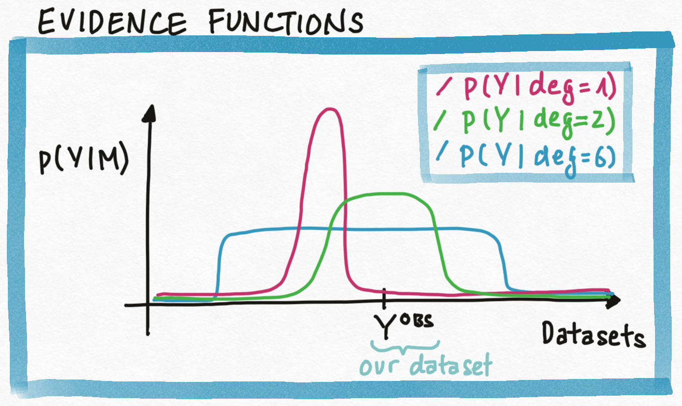
For Bayesian models, there is a natural way to compare different classes of models \(M \in \mathcal{M}\) for a fixed dataset \(Y^{\mathrm{Obs}}\) via the evidence \(p(Y^{\mathrm{Obs}} | M)\), i.e. the average likelihood of the observed data under the models in the prior:
where \(p(\mathbf{w} |M)\) is the prior over the parameters \(\mathbf{w}\) for the model class \(M\).
Since the evidence is a measure of how likely is the data under the model class \(M\), it naturally implies Occam’s Razor - since models from a very complex model classes can generate a wide range datasets, they are unlikely to generate any particular one (our dataset for example); models from very simple model classes are unlikely to fit our data and hence unlikely to generate our dataset.
Model Selection Via Bayes Factor#
Why is this comparison principled? It’s more natural to compare the likelihood of different models given our data, \(p(M|Y^{\mathrm{Obs}})\). For this we need to assume a prior distribution \(p(M)\) over the model classes in \(\mathcal{M}\) and compute the posterior over model classes:
But \(p(Y^{\mathrm{Obs}})\) can’t be computed! So to perform model selection between \(M_1, M_0 \in \mathcal{M}\) we can compute their posterior ratio, which eliminates \(p(Y^{\mathrm{Obs}})\):
When we assume a uniform likelihood over the model classes in \(\mathcal{M}\), this ratio is just \(\frac{p(Y^{\mathrm{Obs}} | M_1)}{p(Y^{\mathrm{Obs}} | M_0)}\), called the Bayes Factor, and it reduces to comparing the evidence of the data under the two models.
Model Selection for Bayesian Models#
But evidence is hard to compute! For Bayesian models we evaluate the predictive accuracy using the (point-wise) log posterior predictive likelihood (lppd) of the observed data:
Again, this is an overestimate of the log-likelihood of new data under the posterior. So a correction must be made. In this case, the correction is the (point-wise) variance of the log posterior predictive likelihood
The Watanabe-Akaike information criterion (WAIC) is defined to be
One may interpret \(p_{\text{WAIC}}\) as an approximation of the effective number of parameters in the model (in a complex hierarchical model the “number of parameters” is not obvious to quantify).
16.3. Inference for General Linear Models#
General Linear Models#
We can add covariates to all the other common statistical models of data \(Y^{(n)} \sim p(Y^{(n)}|\theta^{(n)})\)!
The general scheme is:
Set \(\mathbb{E}[Y^{(n)}] = \theta^{(n)} = g(\mathbf{w}^\top \mathbf{X}^{(n)})\), where \(g\) is typically a non-linear function called the link function (in literature, \(g^{-1}\) is called the link function).
Set the variance according to how the variance of \(p(Y^{(n)}|\theta^{(n)})\) depends on \(\theta\), \(\mathrm{Var}[Y^{(n)}] = \phi f(\theta^{(n)})\), where \(\phi\) is a constant.
These models are called general linear models. Logistic regression is so called because \(g^{-1}\) is the logistic function.
A New Inference Algorithm: Maximum Likelihood by Gradient Descent#
We’d like to learn the parameters \(\mathbf{w}_{\text{MLE}} = \underset{\mathbf{w}}{\mathrm{argmin}} \left(-\ell(\mathbf{w})\right)\). The derivative \(\nabla_\mathbf{w} \left(-\ell(\mathbf{w})\right)\) is easy to derive but hard to solve for stationary points!
Gradient descent: we algorithmically find \(\mathbf{w}^*\) such that the derivative \(\nabla_\mathbf{w} \left(-\ell(\mathbf{w})\right)(\mathbf{w}^*)\) is approximately zero:
start at any \(\mathbf{w}^{(0)}\)
compute: \(\nabla_\mathbf{w} \left(-\ell(\mathbf{w})\right)\) at \(\mathbf{w}^{(current)}\)
take a step in the negative gradient direction:
\[\mathbf{w}^{(new)} \leftarrow \mathbf{w}^{(current)} - \eta * \nabla_\mathbf{w} \left(-\ell(\mathbf{w})\right)(\mathbf{w}^{(current)})\]
We repeat until the derivative is close to zero (stationary).
This algorithm “solves for” the stationary point of \(\nabla_\mathbf{w} \left(-\ell(\mathbf{w})\right)\) for us!
Question: Can we use gradient descent to solve other hard optimization problems we’ve seen in this book?
Subtleties of Gradient Descent: Local vs Global Minima#
If the objective function is convex and the constraints define a convex feasible set, then a stationary point of the objective function gradient or Lagrangian gradient is also a global minimum of the optimization problem.
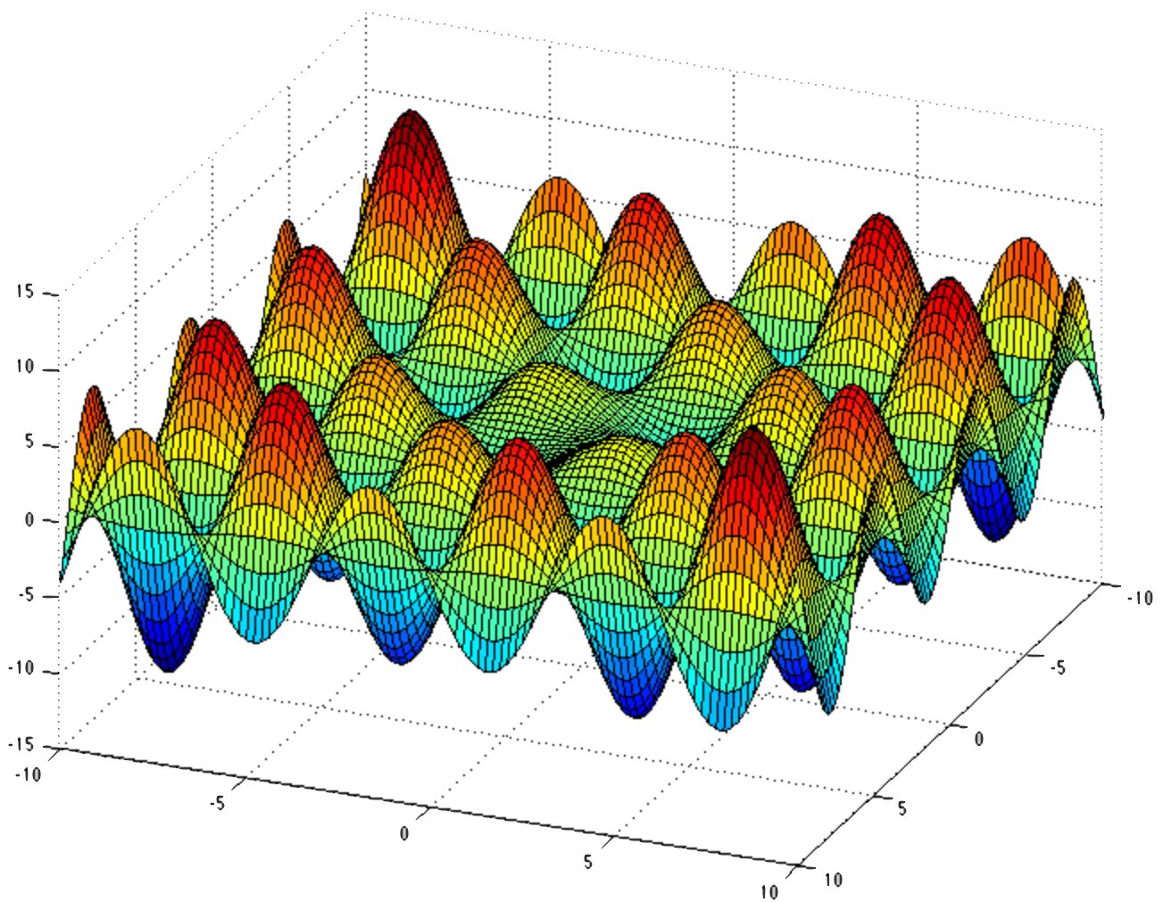
If the optimization problem is nonconvex then there is no guarantee that when gradient descent converges, you’ve found anything close to a global minimum!
Where does Non-Convexity Come From?#
(Link Functions) General linear models with monotone increasing link functions have convex negative log-likelihoods (with respect to a specific parametrization). However, in some cases, we may wish to choose link functions that are not monotone increasing.
(Constraints) Often, we maximize constrained (or regularized) version of the likelihood. These constraints may not always define convex feasible sets.
(Non-Linear Dependency on \(\mathbf{w}\)) In our logistic regression model, \(Y^{(n)} \sim Ber(\mathrm{sigm}(f(\mathbf{X}; \mathbf{w})))\), we can choose a function \(f\) that is non-linear in \(\mathbf{w}\) (it’ll be a neural network later).
Subtleties of Gradient Descent: Scalability#
For every likelihood optimization problem, evaluating the gradient at a set of parameters \(\mathbf{w}\) requires evaluating the likelihood of the entire dataset using \(\mathbf{w}\):
Imagine if the size of your dataset \(N\) is in the millions. Naively evaluating the gradient just once may take up to seconds or minutes, thus running gradient descent until convergence may be unachievable in practice!
Idea: Maybe we don’t need to use the entire data set to evaluate the gradient during each step of gradient descent. Maybe we can approximate the gradient at \(\mathbf{w}\) well enough with just a subset of the data.
16.4. Stochastic Gradient Descent#
Mini-batch Evaluation of the Gradient#
Rather than computing the gradient of the negative log-likelihood at every \(\mathbf{w}\) using the entire dataset, we can approximate the true gradient at \(\mathbf{w}\) by computing the gradient of the negative log-likelihood using a subset of \(N/K\) number of observations.
This modified gradient descent algorithm is called mini-batch gradient descent:
Start at initial value \(\mathbf{w}^{(0)}\).
For
epochs\(= 1, \ldots, \)total_epochs:Shuffle the data and divide up into \(K\)-chunks each with \(N/K\) observations
For \(k =1, \ldots K\):
Compute
grad\((\mathbf{w}) = -\nabla_{\mathrm{w}} \prod_{n=1}^{N/K} p(y^{(n)} |\mathrm{x}^{(n)}, \mathbf{w})\), where \(y^{(n)}, \mathrm{x}^{(n)}\) are from the \(k\)-th chunk.Evaluate
grad\((\mathbf{w}^{(current)})\).Set \(\mathbf{w}^{(new)} \leftarrow \mathbf{w}^{(current)} - \eta *\)
grad\((\mathbf{w}^{(current)})\)
In the extreme case, we choose each chunk to have only 1-observation, the algorithm reduces to randomly selecting an observation to compute the gradient in each iteration.
Mini-batch Evaluation as Stochastic Gradients#
Since the gradient of the negative log-likelihood in each iteration is approximated using a random subset of the data, this approximation introduces stochasticity into the descent algorithm. That is, we can reframe mini-batch gradient descent as stochastic gradient descent:
Start at initial value \(\mathbf{w}^{(0)}\).
Compute: \(\nabla_\mathbf{w} \left(-\ell(\mathbf{w})\right)\) at \(\mathbf{w}^{(current)}\)
Take a stochastic step in the negative gradient direction:
\[\mathbf{w}^{(new)} \leftarrow \mathbf{w}^{(current)} - \eta * \nabla_\mathbf{w} \left(-\ell(\mathbf{w})\right)(\mathbf{w}^{(current)}) + \epsilon\]
where \(\epsilon\sim p(\epsilon)\) is a random variable with mean zero.
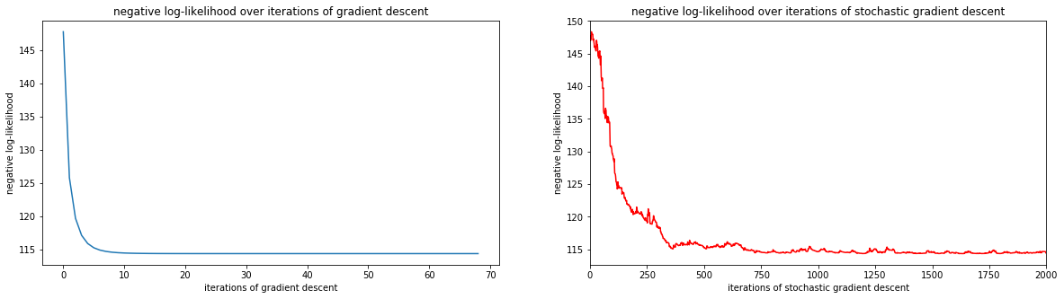
If the negative log-likelihood is convex and we can compute the variance of \(p(\epsilon)\), we can again prove that stochastic gradient descent (and hence mini-batch gradient descent) converges to the global minimum for an appropriate choice of \(\eta\).
Maximum Likelihood with Stochastic Gradient Descent#
What is the difference between the performance of gradient descent and that of stochastic gradient descent on the logistic regression model? Which type of descent should we use for these models?
fig, ax = plt.subplots(1, 2, figsize=(20, 5))
ax = plot_diagnostics(ax, nlls, nlls_s)
plt.show()
16.5. Non-Convex Optimization#
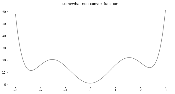
A Non-Convex Optimization Example#
#plot our somewhat non-convex function
fig, ax = plt.subplots(1, 1, figsize=(10, 5))
ax.plot(x, g(x), color='gray')
ax.set_title('somewhat non-convex function')
plt.show()
Gradient Descent for Non-Convex Optimization#
How would gradient descent perform when minimizing a non-convex objective function?
animated_descent
Stochastic Optimization for Non-Convex Optimization#
How would stochastic gradient descent perform when minimizing a non-convex objective function?
aninimated_descent_noisy
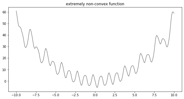
Another Non-Convex Optimization Example#
#plot our extremely non-convex function f
fig, ax = plt.subplots(1, 1, figsize=(10, 5))
ax.plot(x, f(x), color='gray')
ax.set_title('extremely non-convex function')
plt.show()
Stochastic Optimization for Non-Convex Optimization#
How would gradient descent perform when minimizing a non-convex objective function?
aninimated_descent_2
The Idea of Monte Carlo Optimization#
We’ve seen that the randomness of stochastic descent is a desirable feature! The stochasticity can help jump out of local minima. However, since the randomness is uncontrolled (it blindly moves in every direction).
Let’s take inspiration from another stochastic algorithm that blended exploring randomly and exploiting known and highly desirable regions: Metropolis-Hastings.
In MH, random exploration exploration is implemented by a proposal distribution. We always accept if the proposed point is more likely than the current, but sometime we accept a less likely point – this is what allows us to jump to a new region in the sample space.
If our objective function were a pdf, then MH is guaranteed to visit every point with non-zero likelihood asymptotically!
The Idea of Simulated Annealing#
Turn the objective function \(f(x)\) into a pdf \(p(x)\), but with higher mass where \(f\) has lower values. This is the Gibbs distribution:
\[ p(x) \propto \exp\left\{ -\frac{f(x)}{T}\right\},\;\; T \text{ is a constant} \]Note: \(p(x)\) isn’t always a proper pdf!
Use a MH-algorithm with a symmetric proposal distribution to sample values of \(x\) based on \(p(x)\) – MH will be incentivized by \(p(x)\) to sample more \(x\)-values where \(f(x)\) is small! The accept probability is:
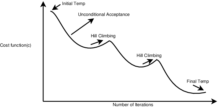
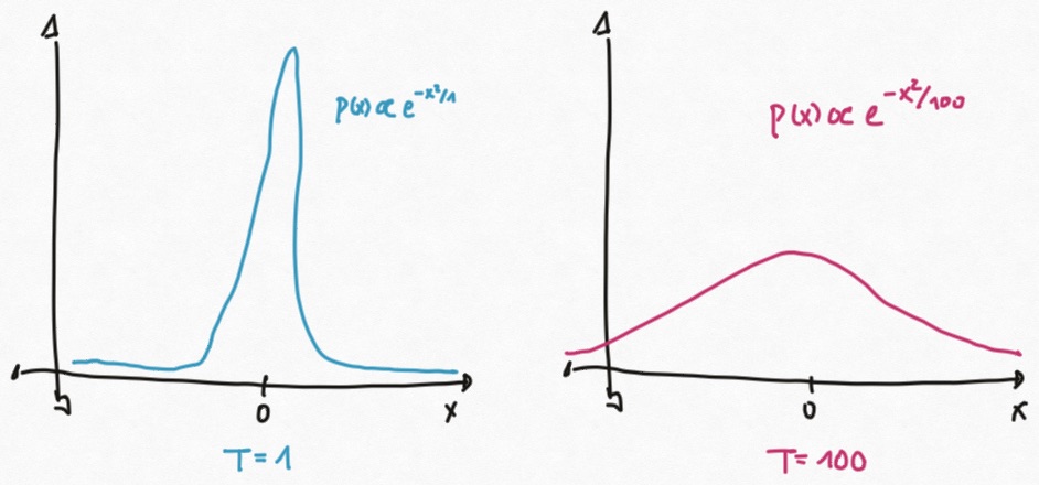
To control exploration vs exploitation, we start with large \(T\) and decrease slowly:
when \(T\) is large, \(\exp\left\{ -\frac{f(x_{\text{proposal}}) - f(x_{\text{old}})}{T}\right\}\) is close to 1
when \(T\) is small, \(\exp\left\{ -\frac{f(x_{\text{proposal}}) - f(x_{\text{old}})}{T}\right\}\) is close to 0 if \(f(x_{\text{proposal}}) > f(x_{\text{old}})\).
Design Choices in Simulated Annealing#
Temperature decreasing schedule
Number of MH-steps to take for each temperature.
As the temperature decreases we should sample more and more. Why?
The Simulated Annealing Algorithm#
initialize anywhere \(x^{(0)}\), initialize temperature
T_0andnumber_of_samplesfor
epoch\(= 1, \ldots\)total_epochsfor
i\(=1, \ldots\)number_of_samplespropose \(x_{\text{proposal}}\) from proposal distribution
compute accept probability \(\alpha(x_{\text{proposal}}, x_{\text{old}})\)
accept \(x_{\text{proposal}}\) or keep \(x_{\text{old}}\) randomly based on \(\alpha(x_{\text{proposal}}, x_{\text{old}})\).
decrease temperature by cooling schedule
increase
number_of_samplesby schedule
Simulated Annealing for Non-Convex Optimization#
#see where the minimum found by SA is
accumulator_sorted = sorted(accumulator, key=lambda t: t[2])
print('we found the minimum of {} at temperature {}'.format(accumulator_sorted[0][2][0], accumulator_sorted[0][0]))
we found the minimum of -5.698015529746401 at temperature 2.097152000000001
aninimated_sa
16.6. Summary#
For a set of observations \(y\), we can collect additional data \(x\) and model the conditional distribution \(p(Y|X)\). This is exactly regression and classification models do, they use covariates \(x\) to predict the outcome \(y\).
(But Sometimes There are Too Many Covariates) The more complicated your model is (e.g. lots of explanatory variables), the more it’ll overfit.
Variable selection by cross-validation of all possible subsets of covariates is not practical. Why?
We can do variable selection by information criteria:
\[\text{*IC} = \underbrace{D(y|\mathbf{w}_{\text{MLE}})}_{\text{(neg) model fit}} + \underbrace{f(\mathrm{dim}(\mathbf{w}_{\text{MLE}}))}_{\text{model complexity}}\]For Bayesian models, we can do variable selection by:
the Bayes factor, i.e. the ratio of the evidence of the data under two different models:
\[ \frac{p(Y^{\mathrm{Obs}} | \text{model 1})}{p(Y^{\mathrm{Obs}} | \text{model 2})}\]WAIC
\[\text{WAIC} = \text{"neg log-likelihood"} + \text{"posterior-variance"}\]
(But the Negative Log Likelihood May Be Highly Non-convex) The more complicated the relationship between \(y\) and \(x\) the more non-convex the negative log-likelihood.
Gradient descent will get trapped often in bad local min
Why does stochastic gradient descent (adding noise to the gradient during descent) help avoid local min? How in practice do we “add noise” to the gradient?
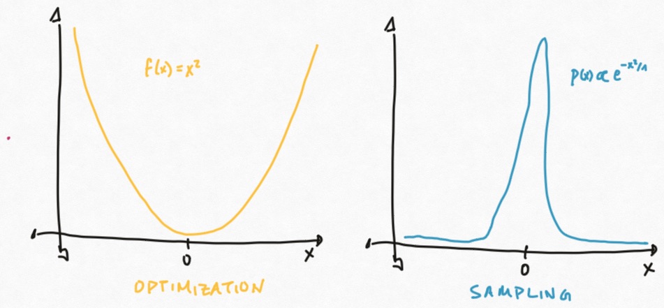
Turn optimization into sampling:
Turn the objective function \(f(x)\) into a pdf \(p(x)\), but with higher mass where \(f\) has lower values. This is the Gibbs distribution:
\[ p(x) \propto \exp\left\{ -\frac{f(x)}{T}\right\},\;\; T \text{ is a constant} \]Sample from \(p(x)\). Wait why is this a good idea?
To control exploration vs exploitation, we start with large \(T\) and decrease slowly. Why?
(With Covariates Comes Greater Explanatory Power) By making the variations in \(y\) explicitly depend on measurable factors \(\mathbf{X}\), we can explain the data in addition to modeling it.
(With Greater Powers Come Greater Problems and Greater Responsibilities) Conditional models have so much potential to generate scientific understanding of our data but they are also the most frequently misused!
(Data Problems) Bias in your conclusions is exponentially exacerbated by bias in the data collection process.
Asking the wrong questions! Wanting information ‘A’ (e.g. sex) but asking a question about ‘B’ (e.g. gender), because we didn’t think carefully about or simply were not aware of the implications of the phrasing of our questions.
This happens because language and semantics about scientific facts change very little or slowly over time, but language and semantics about human experiences are evolving.
Biasing the answers! Offering bad or misrepresentative options as answers, for example, offering an answer option that collapses true variation (e.g. false binaries, overly broad categories).
Violation of user privacy and trust with poor custodianship of sensitive data! For example, not sufficiently protection against data breach, selling sensitive information to 3rd-parties, performing inappropriate profiling and targeting based on sensitive attributes, etc.
These problems can be mitigated by being conscientious and vigilant about the data collection process, and communicating with domain experts as well as affected communities during the entire process!
(Interpretation Problems) It’s tempting (and often easy) to interpret conditional models, but most interpretations are not entirely accurate and can be down right wrong!
Confusing correlation with causation! This can be mitigated by designing follow-up experiments to test for causation!
\[ \underbrace{p(y=1 | x_1, x_2, x_3)}_{\text{$Y$ presence of lung cancer}} = \mathrm{sigm}(-1 + 3 \underbrace{x_1}_{\text{nicotine stains on fingers}} + 1.5 \underbrace{x_2}_{\text{cholestrol}} - 1.75 \underbrace{x_3}_{\text{amount of exercise}}). \]Mis-attribution of importance when covariates are correlated This can be mitigated by performing variable selection!
\[\begin{split}\begin{aligned} (\text{True model})\quad \mathrm{Prob}[\text{Lung Cancer} = 1| \mathbf{X}, \mathbf{w}] &= \mathrm{sigm}(-5 * \text{age} - 0.2 * \text{smoker} - 0.5)\\ (\text{Model where video games (hr) = 0.5 * age})\quad \mathrm{Prob}[\text{Lung Cancer} = 1| \mathbf{X}, \mathbf{w}] &= \mathrm{sigm}(0.5 * \text{age} - 11 * \text{games} - 0.2 * \text{smoker} - 0.5) \end{aligned}\end{split}\]Mis-attribution of importance when the covariates are not equally scaled This can be mitigated by standardizing your data!
\[\begin{aligned} \underbrace{p(y=1 | x_1, x_2, x_3)}_{\text{$Y$ presence of kidney cancer}} = \mathrm{sigm}(-1 + 3 \underbrace{x_1}_{\text{Blood Lead Level g/dL}} + 0.5 \underbrace{x_2}_{\text{HCG in mIU/mL}} - 1.75 \underbrace{x_3}_{\text{Hemo. A1C}}) \end{aligned}\]
(Broader Impact Problems) Because data scientists and machine learning engineers often interact with so many different real-life applications domains (rather than specializing in one domain like medicine or law), we may be the least prepared in terms of domain-specific knowledge but have the greatest impact!
(Not good) Influence on public policy
(Not good) Influence on social and political systems (e.g. Facebook’s internal report on the negative effects of the platform on democratic systems and vulnerable populations)
(Not good) Influence on vulnerable populations
Violation of regulatory statues governing application domains (e.g. fair lending in finance, Title VI in health-care etc)
(We Can Also Accomplish Social Good) It’s not all doom and gloom: while our mistakes (which can happen even when we are vigilant) can be impactful, so can the benefit we might bring. Conditional models can be really useful!
(Personalization) Having explanatory factors for outcomes at the individual level can help personalize treatment and interventions for patients/users.
(Recourse) Having explanatory factors for outcomes at the individual level can help generate recourse (i.e. “what can I do differently”) and empower users to challenge decision making systems.
(Generate scientific hypothesis) Correlation isn’t always causation, but sometimes it is and you discover a new scientific insight!
(Audit black-box decision making systems) Correlation isn’t always causation, but sometimes it is and you discover a bias in the human decision making system that generated the data (e.g. gender and racial biases in everyday language usage uncovered by bias in word embeddings)!
16.7. Exercises#
These problems were originally assigned as homework. Data files are in the book’s data/ folder. Worked solutions, where available, are collapsed beneath the questions they answer; try each problem before expanding them.
Problem Set: Descent Algorithms for Optimization#
Minimizing the Cost of a Construction Project#
Suppose you are building a pricing model for laying down new fibre optics high-speed internet cables under region in the Boston area. Your model takes as input a pair of coordinates, \((x, y)\), and contains two parameters, \(\lambda_1, \lambda_2\). Given a coordinate, \((x, y)\), and model parameters, the loss in revenue corresponding to the price model at location \((x, y)\) is described by
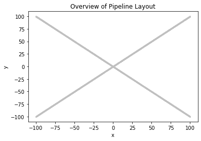
Read the data contained in HW6_data.csv. This is a set of coordinates \(\{(x_n, y_n)\}\) configured on the curve \(y^2 - x^2 = -0.1\). In this problem, we find parameters \(\lambda_1, \lambda_2\) that minimize the net loss over the entire dataset of coordinates \((x_n, y_n)\).
Exercise: Part I: Cost minimization with descent algorithms
(Visualizing the Optimization Landscape) Using level curves (see Chapter 2) and a 3D plot, visually verify that at \(\lambda_1 = 2.05384, \lambda_2 = 0\), the loss function \(L\) is globally minimized.
(Gradient Descent) Implement gradient descent for minimizing the average of \(L\) over the locations given in the data, using the learning rate of 1.0 and initialization of \(\lambda_1 = 2, \lambda_2 = 1\). Visually determine if your algorithm has converged.
Hint: You may need to visualize the behavior over the total number of iterations as well as its value over the last couple of hundreds of iterations to check for convergence.
(Stochastic Gradient Descent) Implement stochastic gradient descent for minimizing the average of \(L\) over the locations in the mini-batch, using the learning rate of 1.0 and initialization of \(\lambda_1 = 2, \lambda_2 = 1\) and mini-batch size of 1. Visually determine if your algorithm has converged.
Hint: You may need to visualize the behavior over the total number of iterations as well as its value over the last couple of hundreds of iterations to check for convergence.
(How to Compare GD and SGD Fairly) Argue that minimizing the average loss over the locations is equivalent to minimizing the net loss. However, minimizing the average loss makes it possible to compare gradient descent and stochastic gradient descent on equal terms. Explain why this is true.
(Comparing the Efficiency of GD and SGD) Compute the average time it takes to update the parameter estimation in each iteration of the two implementations. Which method is faster? Briefly explain why this result should be expected.
Compare the number of iterations it takes for each algorithm to obtain an estimate accurate to
1e-3(in this case, you know the true global optima so you can check the norm \(\|(\lambda_1, \lambda_2) - (\lambda_1^{\text{true}}, \lambda_2^{\text{true}})\|_2\) ). Which method converges to the optimal point in fewer iterations? Briefly explain why this result should be expected.(Comparing Sensitivity of GD and SGD to Learning Rate) Compare the performance of both gradient descent methods for the following learning rates: 1000, 100, 1., 0.1. Based on your observations, briefly describe the effect of the choice of learning rate on the performance of each algorithm. In particular, which algorithm is more sensitive to the learning rate?
Hint: You may need to visualize the behavior over the total number of iterations as well as its value over the first and last couple of hundreds of iterations separately to isolate trends.
(Comparing Sensitivity of GD and SGD to Initialization) Document the behaviour of your two descent algorithms for the following starting points, and for learning rates of 10 and 50:
\((\lambda_1, \lambda_2) = (-2.47865, 0)\)
\((\lambda_1, \lambda_2) = (-3, 0)\)
\((\lambda_1, \lambda_2) = (-5, 0)\)
\((\lambda_1, \lambda_2) = (-10, 0)\)
Based on your visualization of the graph/contour map of the lost function as well as the visualization of the loss function during descent, explain what is happening to your descent algorithms for each initialization.
Solution: Part I, Question 1
### Import basic libraries
import time
import numpy as np
import pandas as pd
import sklearn as sk
import math
from sklearn.linear_model import LinearRegression
import matplotlib.pyplot as plt
from mpl_toolkits.mplot3d import Axes3D
Given our loss function \(L(x, y, \lambda_1, \lambda_2)\) at the coordinate \((x, y)\) and for the set of parameter settings \((\lambda_1, \lambda_2)\), the total loss over the entire set of coordinates in the data is
where \(N\) is total number of coordinates in our data set. Now, since the pipes are being laid down in a particular geometric pattern, namely along a hyperbola described by \(y^2 - x^2 = -0.1\), we can further simplify the above as:
In python, we would write the above as
total_loss = 0.000045 * lambda_2**2 * y.sum() - 0.000098 * lambda_1**2 * x.sum() + 0.003926 * lambda_1 * x.sum() * np.exp(-0.1 * (lambda_1**2 + lambda_2**2))
Now, our task can be stated in a straightforward fashion: we wish to find values of \(\lambda_1\) and \(\lambda_2\) such that the total loss is minimized for our set of coordinates.
Now before running any optimization algorithms on our objective function, we must do some exploration of our function, either by analysis or visualization! This step is important for the following reasons:
iteratively following the gradient (the direction of maximum increase or decrease in the objective function at a point) does not guarantee that you will end in a global maximum or minimum. In fact, if your function has local maxima, local minima or saddle points (at which the gradient is zero - these are called stationary points), your gradient descent may very well become trapped at these points. In this sense, where you initialize your gradient descent algorithm becomes very important. Some initializations will lead you to an undesirable stationary point, while others will lead you to your global maximum or minimum.
analytical, numerical or visual explorations of your function can help you determine appropriate step sizes for your descent algorithms (would \(\eta = 0.001\) be appropriate or \(\eta=1000\)?).
#Visualization of the data - what does the pipeline look like?
x, y = np.genfromtxt('../data/HW6_data.csv', delimiter=',')

plt.scatter(x, y, color='silver', s=1)
plt.xlabel('x')
plt.ylabel('y')
plt.title('Overview of Pipeline Layout')
plt.show()
x_sum = x.sum()
y_sum = y.sum()
N = len(x)

#define total loss
L = lambda l1, l2, x, y: 0.000045 * l2**2 * y.sum() - 0.000098 * l1**2 * x.sum() + 0.003926 * x.sum() * l1 * np.exp(-0.1 * (l1**2 + l2**2))
#cover the domain of the pdf with a grid and get the coordinates of the grid vertices
delta = 0.25
l1 = np.arange(-10, 10, delta)
l2 = np.arange(-10, 10, delta)
l1, l2 = np.meshgrid(l1, l2)

loss = L(l1, l2, x, y)

fig = plt.figure(figsize=(15, 5))


#plot contour map of pdf with data in R^2 (Cartesian plane)
ax1 = fig.add_subplot(121)
contour = ax1.contour(l1, l2, loss, levels=np.linspace(-10, 30, 20))
ax1.scatter([2.05384], [0], color='red', s=50, label='global min @ (2.05384, 0)')
ax1.clabel(contour, inline=1, fontsize=10)
ax1.set_title('Contour Graph of Loss Function with Minimum Solution')
ax1.set_xlabel('lambda_1')
ax1.set_ylabel('lambda_2')
ax1.legend(loc='best')

#plot 3D suface of pdf in R^3
ax2 = fig.add_subplot(122, projection='3d')
ax2.plot_trisurf(l1.flatten(), l2.flatten(), loss.flatten(), linewidth=0.2, antialiased=True, color='skyblue', alpha=0.8)
ax2.scatter([2.05384], [0], [L(2.05384, 0, x, y)], color='red', s=50, label='global min @ (2.05384, 0)')
ax2.set_xlabel('lambda_1')
ax2.set_ylabel('lambda_2')
ax2.set_zlabel('total loss')
ax2.set_title('Graph of Loss Function with Minimum Solution')
ax2.legend(loc='best')

plt.show()
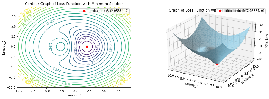
From the above, we see that the total loss is minimized at \((\lambda_1, \lambda_2) = (2.05384, 0)\). We leave to you to find the other points of interest in the parameter space (it is important that you do!).
print('The minumum total cost:', L(2.05384, 0, x, y))
The minumum total cost: -9.934104025304476
Disclaimer: A negative total is not very interpretable from a business perspective but this is what we are working with.
Solution: Part I, Question 2
We first calculate the gradient of our total loss function,
#The gradient of the total loss function
grad = lambda l1, l2, x, y: np.array([-0.000098 * 2 * l1 * x.sum()
                                      + 0.003926 *  x.sum() * np.exp(-0.1 * (l1**2 + l2**2))
                                      - 0.003926 * 2 * 0.1 *  x.sum() * l1**2 * np.exp(-0.1 * (l1**2 + l2**2)),
                                      2 * 0.000045 * l2 * y.sum()
                                      - 0.1 * 2* 0.003926 *  x.sum() * l1 * l2 * np.exp(-0.1 * (l1**2 + l2**2))])
A note on the correct stopping condition to use:
Average/Total loss or lambdas? In this problem, we know the precise location of the global minimum: (2.05384, 0), and we know the minimum total cost: -9.9341040253. So should we stop when we are sufficiently close to the optimal parameters, \((2.05384, 0)\), or should we stop when we are sufficiently close to the minimum total cost? Well, the difference is not significant and in general you can choose to use either as your stopping condition. However, since evaluating the cost at each step of the gradient descent (which involves summing over your entire dataset) is one extra computation expense, it might be more efficient to use distance to the optimal parameters as your stopping condition.
That is, we stop our descent when
where \(\| \cdot \|_2\) is the \(\ell_2\) norm or the Euclidean distance.
#Gradient Descent
def gradient_descent(x, y, lambdas_init, init_shuffle=False, step_size=0.001, maxsteps=None, precision=1e-3):

    lambdas = lambdas_init
    history = [lambdas] # to store all parameters
    grad_norms = [np.linalg.norm(grad(lambdas[0], lambdas[1], x, y) * 1. / N)]
    counter = 0

    #if you want to shuffle the data before doing descent
    if init_shuffle:
        shuffle = np.random.permutation(N)
        x = x[shuffle]
        y = y[shuffle]

    #Do descent while stopping condition not met
    while np.linalg.norm(history[-1] - np.array([2.05384, 0])) > precision:
        #get gradient of average loss function
        gradient = grad(lambdas[0], lambdas[1], x, y) * 1. / N
        #take one step in the gradient direction
        lambdas = lambdas -  step_size * gradient
        #add our new parameters to the history
        history.append(lambdas)
        #add the norm of the gradient to our list of norms
        grad_norms.append(np.linalg.norm(gradient))
        #tick off one more step
        counter +=1

        #if we've hit maximum steps allowed, stop!
        if maxsteps is not None:
            if counter == maxsteps:
                break

    return history, grad_norms
lambdas_init = [2, 1]
start = time.time()
grad(lambdas_init[0], lambdas_init[1], x, y) * 1./len(x)
end = time.time()

history, grad_norms_gd = gradient_descent(x, y, lambdas_init, step_size=1., maxsteps=100000)
history = np.array(history)

lambdas = history[-1]
costs = L(history[:, 0], history[:, 1], x, y)

print('time to compute one gradient: ', end - start)
print('how many iters: ', len(history))
print('final cost:', costs[-1])
print('precision to actual param:', np.linalg.norm(lambdas - [2.05384, 0]))

fig, ax = plt.subplots(1, 2, figsize=(20, 5))
ax[0].plot(range(len(costs)), costs, label='total cost vs iteration')
ax[0].set_xlabel('iteration')
ax[0].set_ylabel('total cost')
ax[0].set_title('Total Cost vs Iteration in Gradient Descent')
ax[0].legend(loc='best')

ax[1].plot(range(len(costs)), grad_norms_gd, color='red')
ax[1].set_title('Gradient Norms During Descent')
plt.show()
time to compute one gradient:  0.0003361701965332031
how many iters:  43545
final cost: -9.93410274854933
precision to actual param: 0.000999868898540722
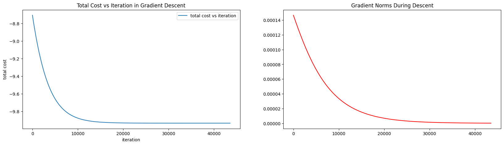
We see that we are within tolerance of our optimal parameters after 43,545 steps in the gradient descent algorithm. From the visualization of the total cost versus iteration, we see that initially we were making large updates to our parameters (the total cost was changing quickly), but towards the end the updates to our parameters became smaller and smaller (the total cost was not changing very much from iteration to iteration). This is expected, as the gradient around the global minimum in our case should be close to zero, resulting in very small step-sizes in our descent.
Solution: Part I, Question 3
The algorithm for Stochastic Gradient Descent is nearly identical to gradient descent, except for the fact that when we compute the gradient, we feed the gradient function a single coordinate rather than the entire dataset. Furthermore, we make multiple passes through the data, randomizing the dataset at the beginning each time.
#Stochastic Gradient Descent
def sgd(x, y, lambdas_init, init_shuffle=False, step_size=0.001, max_epochs=1, precision=1e-3, output=True):
    lambdas = lambdas_init
    history = [lambdas] # to store all thetas
    grad_norms = [np.linalg.norm(grad(lambdas[0], lambdas[1], x, y) * 1. / N)]
    counter = 0
    epochs = 0
    i = 0 #index

    #if you want to shuffle the data before doing descent
    if init_shuffle:
        shuffle = np.random.permutation(N)
        x = x[shuffle]
        y = y[shuffle]

    #run through the data in multiple passes
    for epoch in range(max_epochs):
        #for each data point, compute the gradient and make an update to our parameters
        if output == True:
            print('epoch: ', epoch)
        for i in range(N):
            #get gradient of average loss function
            gradient = grad(lambdas[0], lambdas[1], x[i], y[i])
            #take one step in the gradient direction
            lambdas = lambdas -  step_size * gradient
            #add our new parameters to the history
            history.append(lambdas)
            #add the norm of the gradient to our list of norms
            grad_norms.append(np.linalg.norm(gradient))

            if np.linalg.norm(np.array(lambdas) - np.array([2.05384, 0])) < precision:
                return history, epoch, grad_norms
            elif np.any(np.isnan(lambdas)):
                return history[:-1], epoch, grad_norms

        #shuffle the data for the next pass thru
        shuffle = np.random.permutation(N)
        x = x[shuffle]
        y = y[shuffle]

    return history, max_epochs, grad_norms
lambdas_init = [2, 1]
start = time.time()
grad(lambdas_init[0], lambdas_init[1], x[0], y[0])
end = time.time()

history, epoch, grad_norms_sgd = sgd(x, y, lambdas_init, init_shuffle=False, step_size=1., max_epochs=8)
history = np.array(history)

lambdas = history[-1]
costs = L(history[:, 0], history[:, 1], x, y)
print('****************************')
print('no initial random shuffling')
print('****************************')
print('time to compute one gradient: ', end - start)
print('how many iters: ', len(history))
print('final loss:', costs[-1])
print('precision to actual param:', np.linalg.norm(lambdas - [2.05384, 0]))

fig, ((ax1, ax2), (ax3, ax4)) = plt.subplots(2, 2, figsize=(20, 10))

ax1.plot(range(len(costs)), costs, label='total cost vs iteration')
ax1.set_xlabel('iteration')
ax1.set_ylabel('total loss')
ax1.set_title('Total Loss vs Iteration in Stochastic Gradient Descent')
ax1.legend(loc='best')

ax2.plot(np.arange(len(costs) - 100, len(costs)), costs[-100:], label='total cost vs iteration')
ax2.set_xlabel('iteration')
ax2.set_ylabel('total loss')
ax2.set_title('Total Loss vs Iteration in Stochastic Gradient Descent (Last 100 Iterations)')
ax2.legend(loc='best')

ax3.plot(range(len(costs)), grad_norms_sgd, color='red')
ax3.set_title('Gradient Norms During Descent')

ax4.plot(range(15000, len(costs)), grad_norms_sgd[15000:], color='red')
ax4.set_title('Gradient Norms During Descent During the End of the Descent')
plt.show()
epoch:  0
****************************
no initial random shuffling
****************************
time to compute one gradient:  4.100799560546875e-05
how many iters:  15868
final loss: -9.934102852275833
precision to actual param: 0.0009584050556876609
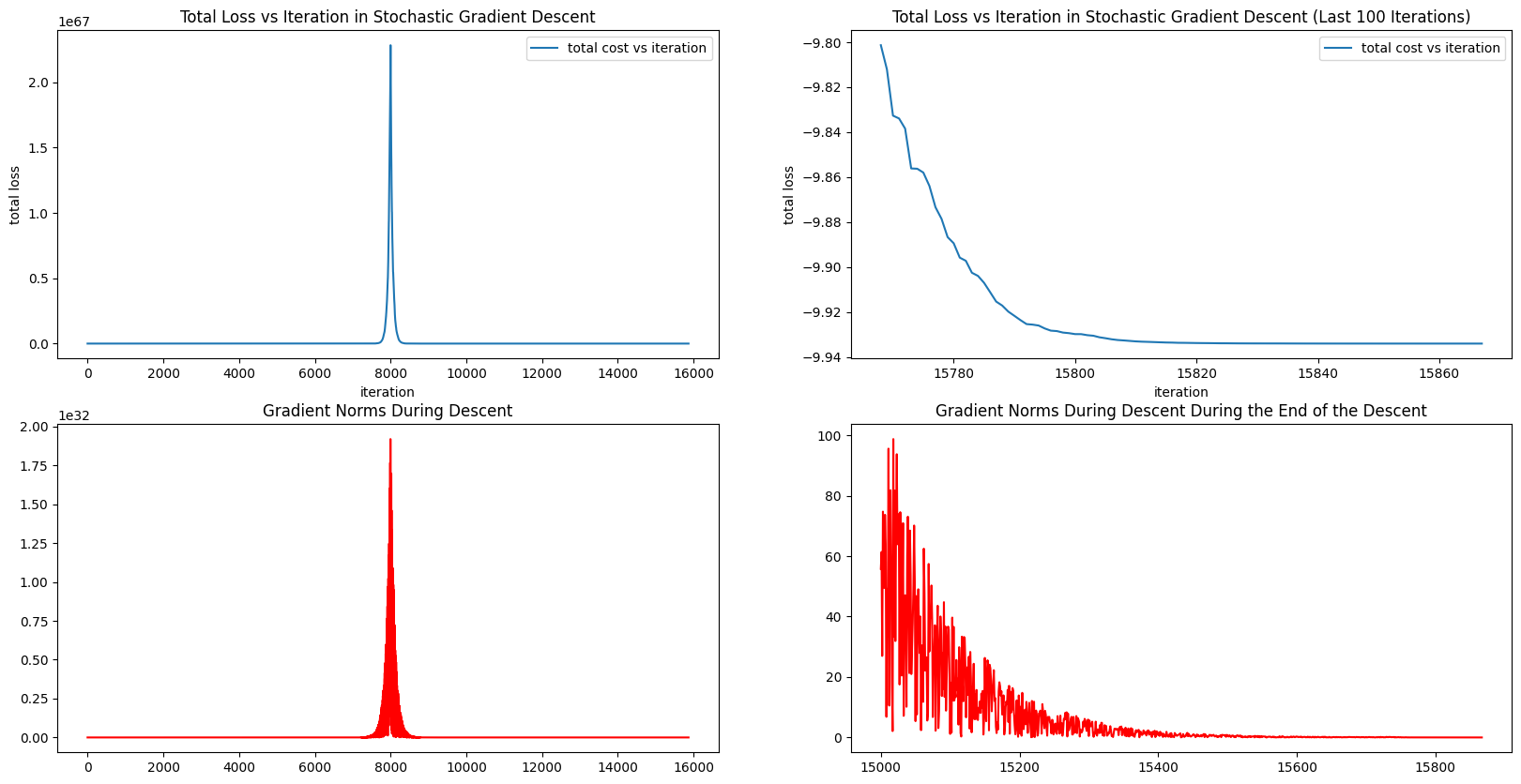
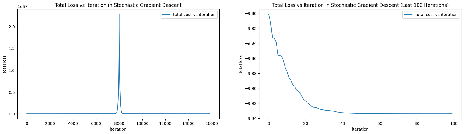
We see that we are within tolerance of our optimal parameters after 15,868 steps (versus the 43,545 steps it takes gradient descent) in the stochastic gradient descent algorithm. From the visualization of the total loss versus iteration, we see that during our descent, we headed (around iteration number 8,000) in the direction which increased total cost! But how can this happen?
Recall that in stochastic gradient descent, we are stepping in the direction that minimizes the loss function for just one data point rather than the direction that minimized the loss over the entire dataset. Clearly, pursuing local, short term gains does not lead you down the same path as pursuing global, long term gains. Thus, descending in the direction that decreases the loss for one data point can often lead to an increase the loss over the entire dataset.
Interestingly enough, although our total loss spiked around iteration 8,000, our stochastic gradient descent was able to find the global minimum in a shorter total number of iterations! That is, sometimes the quickest way down hill lies beyond a big climb!
In contrast, gradient descent is typically incapable of finding paths along which the total cost rises. That is, the total cost is expected to decrease from one iteration to the next.
Another thing to note is that the gradient norms of SGD tend to be quite large compared with those of gradient descent. While it’s not always good to have a large gradient norm, if the steps taken by a descent algorithm are towards a good direction, then large steps can lead to faster convergence.
lambdas_init = [2, -1]
start = time.time()
grad(lambdas_init[0], lambdas_init[1], x[0], y[0])
end = time.time()

history, epoch, grad_norms_sgd = sgd(x, y, lambdas_init, init_shuffle=True, step_size=1., max_epochs=8)
history = np.array(history)

lambdas = history[-1]
costs = L(history[:, 0], history[:, 1], x, y)
print('****************************')
print('with initial random shuffling')
print('****************************')
print('time to compute one gradient: ', end - start)
print('how many iters: ', len(history))
print('final loss:', costs[-1])
print('precision to actual param:', np.linalg.norm(lambdas - [2.05384, 0]))

fig, ((ax1, ax2), (ax3, ax4)) = plt.subplots(2, 2, figsize=(20, 10))

ax1.plot(range(len(costs)), costs, label='total cost vs iteration')
ax1.set_xlabel('iteration')
ax1.set_ylabel('total loss')
ax1.set_title('Total Loss vs Iteration in Stochastic Gradient Descent')
ax1.legend(loc='best')

ax2.plot(np.arange(len(costs) - 100, len(costs)), costs[-100:], label='total cost vs iteration')
ax2.set_xlabel('iteration')
ax2.set_ylabel('total loss')
ax2.set_title('Total Loss vs Iteration in Stochastic Gradient Descent (Last 100 Iterations)')
ax2.legend(loc='best')

ax3.plot(range(len(costs)), grad_norms_sgd, color='red')
ax3.set_title('Gradient Norms During Descent')

ax4.plot(np.arange(len(costs) - 500, len(costs)), grad_norms_sgd[-500:], color='red')
ax4.set_title('Gradient Norms During Descent During the End of the Descent')
plt.show()
epoch:  0
****************************
with initial random shuffling
****************************
time to compute one gradient:  4.1961669921875e-05
how many iters:  5637
final loss: -9.934102757824299
precision to actual param: 0.0009962336310606358
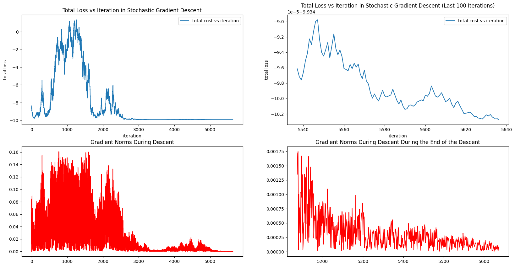
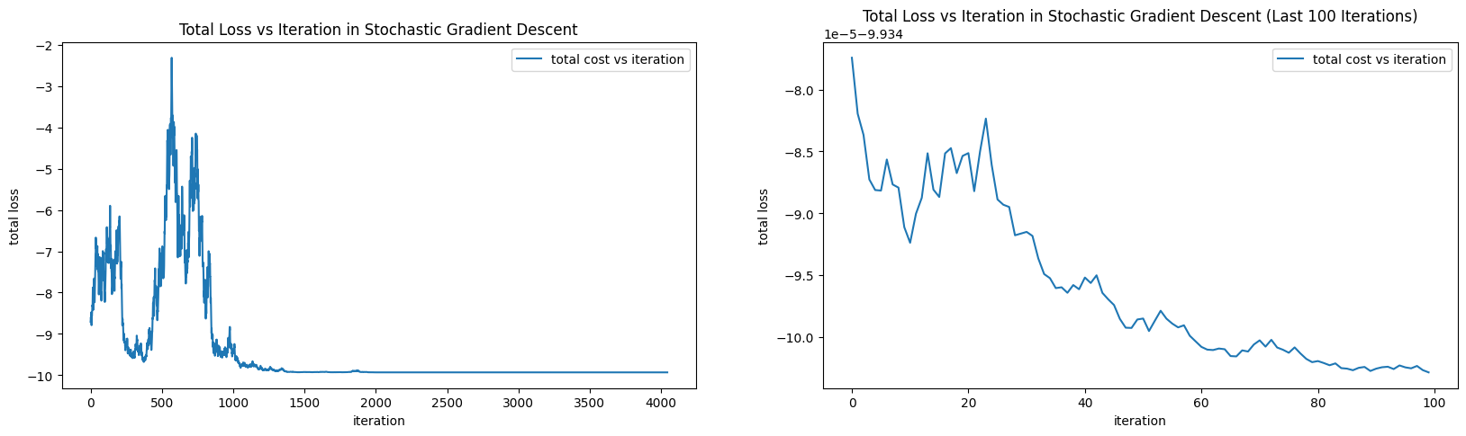
We see that we are within tolerance of our optimal parameters after 5,637 steps (versus the 43,545 steps it takes gradient descent) in the stochastic gradient descent algorithm. From the visualization of the total loss versus iteration, we see that, with an initial shuffling of the data, the path stochastic gradient descent takes to the optimal solution is even more erratic. We are taking paths along which the total loss rises and drops before finally stabilizing somewhat around the optimal total loss of -9.9341.
Again, the gradient norms of SGD tend to be quite large compared with those of gradient descent. Again, it’s not always good to have a large gradient norm, but in this case, we see that the steps taken by sgd are always towards the direction of the global min, thus the large steps lead to faster convergence.
When we examine the total loss for the last 100 iterations, we see that stochastic gradient descent is oscillating around the optimal loss. This behaviour can be worrisome if we need to obtain a higher precision solution - it’s possible that stochastic gradient descent will never fall within the required tolerance.
Solution: Part I, Question 4
Total Loss or Average Loss? If we’re just interested in minimizing the loss, minimizing total loss is equivalent to minimizing average loss. This is because
Clearly, since \(N\) is a constant, when total loss is minimized then average loss is minimized (and vice versa). However, if we are interested in comparing the performance of gradient descent with that of stochastic gradient descent, we need to find a loss function that facilitates a fair comparison.
If we use the total loss for both descent algorithm, then the gradient for gradient descent will tend to be much larger (since in gradient descent, we sum over the entire dataset to compute the gradient, whereas in stochastic gradient descent, we use only one pair of coordinates to compute the gradient). Larger gradients will tend to yield larger steps in our descent, which, in turn, will tend to result in faster convergence.
To be fair, we will use the average loss function for both gradient descent and stochastic gradient descent. This make sense semantically as well, the loss function averaged over the entire data set is the expected loss for a single coordinate, whereas evaluating the loss function at a random coordinate is a way of approximating the expected loss for a single coordinate.
Coding wise, we just need to multiply the total cost function and the gradient function we’ve defined by 1/N to turn them into averages.
Solution: Part I, Question 5
In the runs above, it takes about 0.00034 seconds to compute one gradient for gradient descent, while it takes around 0.00004 seconds to compute one gradient for stochastic gradient descent. This is expected. We expect that computing gradients for gradient descent can take longer, given that we must perform operations on the entire set of data. However, since our dataset is relatively small and our operations (sums) are relatively light weight, the difference between these two gradient computations is minute.
However, this will not always be the case (i.e. our data will not always be small, and the operations required to compute the gradient will not always be simple)!
So is Stochastic Gradient Descent a faster algorithm? To answer this question rigorously and productively, we must decompose our notion of fast in two ways:
the time it takes to compute one gradient
the number of steps it takes to converge to an acceptable solution
We’ve already addressed the difficulty of computing the gradient over the entire dataset - in this case, stochastic gradient descent is the “faster” algorithm. In our case stochastic gradient descent found the global optimum in fewer iterations. However, this is an exception. We can already see, from our visualizations, that stochastic gradient descent can take paths through the parameter space that increases total cost, and it can have oscillating behaviour when it approaches the global optima. In fact, the erratic paths SGD takes can often lead to slow convergence and the algorithm can easily fail to converge at all (i.e. never being able to achieve a certain degree to accuracy).
Solution: Part I, Question 6
So how does a change in step size affect the performance of stochastic gradient descent? We will run SGD for various stepsize, each time testing the step size with an initial randomization of the data and without.
lambdas_init = [2, -1]
start = time.time()
grad(lambdas_init[0], lambdas_init[1], x[0], y[0])
end = time.time()

step_sizes = [0.1, 1., 100, 1000.]

fig, ax = plt.subplots(1, 4, figsize=(24, 5))

for i in range(len(step_sizes)):
    step_size = step_sizes[i]
    history, _ = gradient_descent(x, y, lambdas_init, step_size=step_size, maxsteps=100000)
    history = np.array(history)
    costs = L(history[:, 0], history[:, 1], x, y)

    ax[i].plot(range(len(costs)), costs, label='total cost vs iteration')
    ax[i].set_xlabel('iteration')
    ax[i].set_ylabel('total loss')
    ax[i].set_title('Gradient Descent, step size {}'.format(step_size))
    ax[i].legend(loc='best')

plt.show()
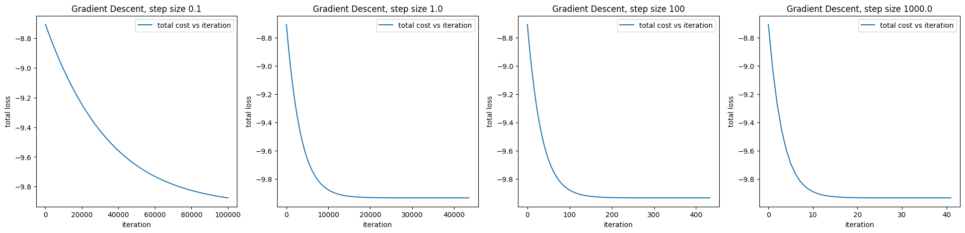
It doesn’t look like gradient descent is too sensitive to the step size (at least from the initialization we chose).
lambdas_init = [2, -1]
start = time.time()
grad(lambdas_init[0], lambdas_init[1], x[0], y[0])
end = time.time()

step_size = 0.1

history, epoch, _ = sgd(x, y, lambdas_init, init_shuffle=False, step_size=step_size, max_epochs=8)
history = np.array(history)

lambdas = history[-1]
costs = L(history[:, 0], history[:, 1], x, y)
print('****************************')
print('without initial random shuffling')
print('****************************')
print('stepsize: ', step_size)
print('time to compute one gradient: ', end - start)
print('how many iters: ', len(history))
print('final loss:', costs[-1])
print('precision to actual param:', np.linalg.norm(lambdas - [2.05384, 0]))

fig, (ax1, ax2) = plt.subplots(1, 2, figsize=(20, 5))

ax1.plot(range(len(costs)), costs, label='total cost vs iteration')
ax1.set_xlabel('iteration')
ax1.set_ylabel('total loss')
ax1.set_title('Total Loss vs Iteration in Stochastic Gradient Descent')
ax1.legend(loc='best')

ax2.plot(range(len(costs[-100:])), costs[-100:], label='total cost vs iteration')
ax2.set_xlabel('iteration')
ax2.set_ylabel('total loss')
ax2.set_title('Total Loss vs Iteration in Stochastic Gradient Descent (Last 100 Iterations)')
ax2.legend(loc='best')
plt.show()
epoch:  0
epoch:  1
epoch:  2
epoch:  3
epoch:  4
epoch:  5
epoch:  6
epoch:  7
****************************
without initial random shuffling
****************************
stepsize:  0.1
time to compute one gradient:  3.5762786865234375e-05
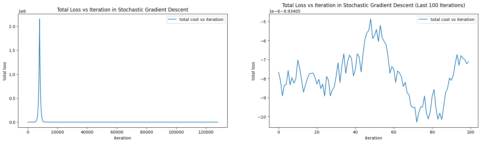
how many iters:  128001
final loss: -9.934057116634932
precision to actual param: 0.006059913435087186
lambdas_init = [2, -1]
start = time.time()
grad(lambdas_init[0], lambdas_init[1], x[0], y[0])
end = time.time()

step_size = 0.1

history, epoch, _ = sgd(x, y, lambdas_init, init_shuffle=True, step_size=step_size, max_epochs=8)
history = np.array(history)

lambdas = history[-1]
costs = L(history[:, 0], history[:, 1], x, y)
print('****************************')
print('with initial random shuffling')
print('****************************')
print('stepsize: ', step_size)
print('time to compute one gradient: ', end - start)
print('how many iters: ', len(history))
print('final loss:', costs[-1])
print('precision to actual param:', np.linalg.norm(lambdas - [2.05384, 0]))

fig, (ax1, ax2) = plt.subplots(1, 2, figsize=(20, 5))

ax1.plot(range(len(costs)), costs, label='total cost vs iteration')
ax1.set_xlabel('iteration')
ax1.set_ylabel('total loss')
ax1.set_title('Total Loss vs Iteration in Stochastic Gradient Descent')
ax1.legend(loc='best')

ax2.plot(range(len(costs[-100:])), costs[-100:], label='total cost vs iteration')
ax2.set_xlabel('iteration')
ax2.set_ylabel('total loss')
ax2.set_title('Total Loss vs Iteration in Stochastic Gradient Descent (Last 100 Iterations)')
ax2.legend(loc='best')
plt.show()
epoch:  0
epoch:  1
epoch:  2
epoch:  3
epoch:  4
epoch:  5
epoch:  6
epoch:  7
****************************
with initial random shuffling
****************************
stepsize:  0.1
time to compute one gradient:  3.6716461181640625e-05
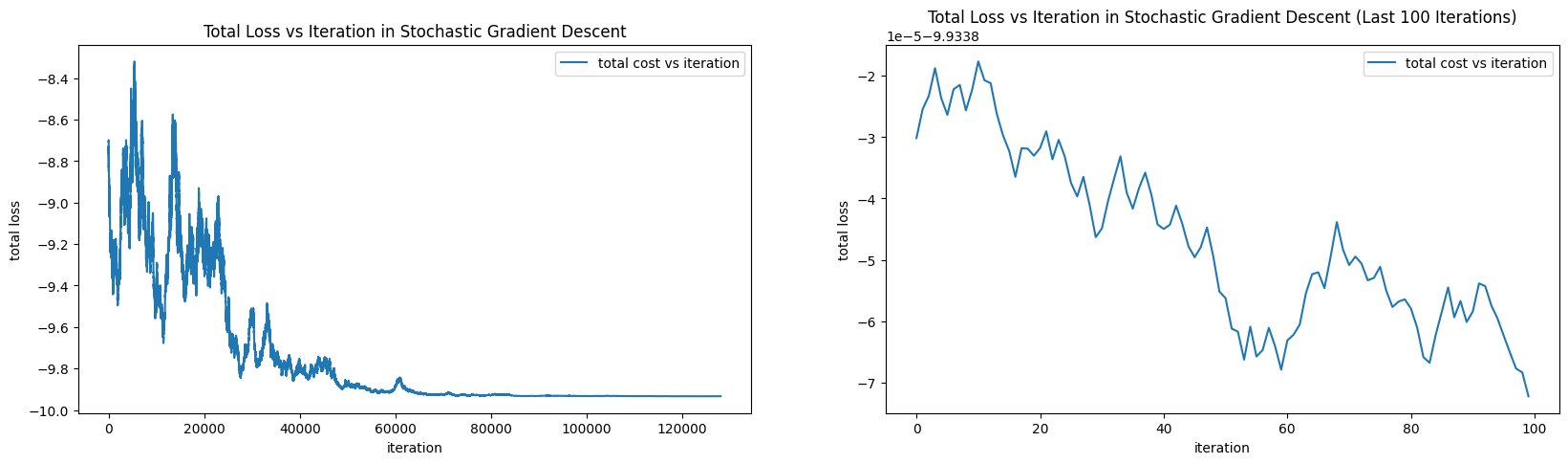
how many iters:  128001
final loss: -9.93387224694684
precision to actual param: 0.013470277064085552
lambdas_init = [2, -1]
start = time.time()
grad(lambdas_init[0], lambdas_init[1], x[0], y[0])
end = time.time()

step_size = 1.

history, epoch, _ = sgd(x, y, lambdas_init, init_shuffle=False, step_size=step_size, max_epochs=8)
history = np.array(history)

lambdas = history[-1]
costs = L(history[:, 0], history[:, 1], x, y)
print('****************************')
print('without initial random shuffling')
print('****************************')
print('stepsize: ', step_size)
print('time to compute one gradient: ', end - start)
print('how many iters: ', len(history))
print('final loss:', costs[-1])
print('precision to actual param:', np.linalg.norm(lambdas - [2.05384, 0]))

fig, (ax1, ax2) = plt.subplots(1, 2, figsize=(20, 5))

ax1.plot(range(len(costs)), costs, label='total cost vs iteration')
ax1.set_xlabel('iteration')
ax1.set_ylabel('total loss')
ax1.set_title('Total Loss vs Iteration in Stochastic Gradient Descent')
ax1.legend(loc='best')

ax2.plot(range(len(costs[-100:])), costs[-100:], label='total cost vs iteration')
ax2.set_xlabel('iteration')
ax2.set_ylabel('total loss')
ax2.set_title('Total Loss vs Iteration in Stochastic Gradient Descent (Last 100 Iterations)')
ax2.legend(loc='best')
plt.show()
epoch:  0
****************************
without initial random shuffling
****************************
stepsize:  1.0
time to compute one gradient:  3.886222839355469e-05
how many iters:  15868
final loss: -9.934102852275833
precision to actual param: 0.0009584050556876609
lambdas_init = [2, -1]
start = time.time()
grad(lambdas_init[0], lambdas_init[1], x[0], y[0])
end = time.time()

step_size = 1.

history, epoch, _ = sgd(x, y, lambdas_init, init_shuffle=True, step_size=step_size, max_epochs=8)
history = np.array(history)

lambdas = history[-1]
costs = L(history[:, 0], history[:, 1], x, y)
print('****************************')
print('with initial random shuffling')
print('****************************')
print('stepsize: ', step_size)
print('time to compute one gradient: ', end - start)
print('how many iters: ', len(history))
print('final loss:', costs[-1])
print('precision to actual param:', np.linalg.norm(lambdas - [2.05384, 0]))

fig, (ax1, ax2) = plt.subplots(1, 2, figsize=(20, 5))

ax1.plot(range(len(costs)), costs, label='total cost vs iteration')
ax1.set_xlabel('iteration')
ax1.set_ylabel('total loss')
ax1.set_title('Total Loss vs Iteration in Stochastic Gradient Descent')
ax1.legend(loc='best')

ax2.plot(range(len(costs[-100:])), costs[-100:], label='total cost vs iteration')
ax2.set_xlabel('iteration')
ax2.set_ylabel('total loss')
ax2.set_title('Total Loss vs Iteration in Stochastic Gradient Descent (Last 100 Iterations)')
ax2.legend(loc='best')
plt.show()
epoch:  0
****************************
with initial random shuffling
****************************
stepsize:  1.0
time to compute one gradient:  3.314018249511719e-05
how many iters:  4045
final loss: -9.934102854819784
precision to actual param: 0.0009573656086993795
lambdas_init = [2, -1]
start = time.time()
grad(lambdas_init[0], lambdas_init[1], x[0], y[0])
end = time.time()

step_size = 100.

history, epoch, _ = sgd(x, y, lambdas_init, init_shuffle=False, step_size=step_size, max_epochs=8)
history = np.array(history)

lambdas = history[-1]
costs = L(history[:, 0], history[:, 1], x, y)
print('****************************')
print('without initial random shuffling')
print('****************************')
print('stepsize: ', step_size)
print('time to compute one gradient: ', end - start)
print('how many iters: ', len(history))
print('final loss:', costs[-1])
print('precision to actual param:', np.linalg.norm(lambdas - [2.05384, 0]))

fig, (ax1, ax2) = plt.subplots(1, 2, figsize=(20, 5))

ax1.plot(range(len(costs)), costs, label='total cost vs iteration')
ax1.set_xlabel('iteration')
ax1.set_ylabel('total loss')
ax1.set_title('Total Loss vs Iteration in Stochastic Gradient Descent')
ax1.legend(loc='best')

ax2.plot(range(len(costs[-100:])), costs[-100:], label='total cost vs iteration')
ax2.set_xlabel('iteration')
ax2.set_ylabel('total loss')
ax2.set_title('Total Loss vs Iteration in Stochastic Gradient Descent (Last 100 Iterations)')
ax2.legend(loc='best')
plt.show()
epoch:  0
****************************
without initial random shuffling
****************************
stepsize:  100.0
time to compute one gradient:  3.314018249511719e-05
how many iters:  541
final loss: inf
precision to actual param: inf
lambdas_init = [2, -1]
start = time.time()
grad(lambdas_init[0], lambdas_init[1], x[0], y[0])
end = time.time()

step_size = 100.

history, epoch, _ = sgd(x, y, lambdas_init, init_shuffle=True, step_size=step_size, max_epochs=8)
history = np.array(history)

lambdas = history[-1]
costs = L(history[:, 0], history[:, 1], x, y)
print('****************************')
print('with initial random shuffling')
print('****************************')
print('stepsize: ', step_size)
print('time to compute one gradient: ', end - start)
print('how many iters: ', len(history))
print('final loss:', costs[-1])
print('precision to actual param:', np.linalg.norm(lambdas - [2.05384, 0]))

fig, (ax1, ax2) = plt.subplots(1, 2, figsize=(20, 5))

ax1.plot(range(len(costs)), costs, label='total cost vs iteration')
ax1.set_xlabel('iteration')
ax1.set_ylabel('total loss')
ax1.set_title('Total Loss vs Iteration in Stochastic Gradient Descent')
ax1.legend(loc='best')

ax2.plot(range(len(costs[-100:])), costs[-100:], label='total cost vs iteration')
ax2.set_xlabel('iteration')
ax2.set_ylabel('total loss')
ax2.set_title('Total Loss vs Iteration in Stochastic Gradient Descent (Last 100 Iterations)')
ax2.legend(loc='best')
plt.show()
epoch:  0
epoch:  1
epoch:  2
epoch:  3
epoch:  4
****************************
with initial random shuffling
****************************
stepsize:  100.0
time to compute one gradient:  3.504753112792969e-05
how many iters:  72058
final loss: -9.93410396538139
precision to actual param: 0.0001453783488463145
lambdas_init = [2, -1]
start = time.time()
grad(lambdas_init[0], lambdas_init[1], x[0], y[0])
end = time.time()

step_size = 1000.

history, epoch, _ = sgd(x, y, lambdas_init, init_shuffle=True, step_size=step_size, max_epochs=8)
history = np.array(history)

lambdas = history[-1]
costs = L(history[:, 0], history[:, 1], x, y)
print('****************************')
print('with initial random shuffling')
print('****************************')
print('stepsize: ', step_size)
print('time to compute one gradient: ', end - start)
print('how many iters: ', len(history))
print('final loss:', costs[-1])
print('precision to actual param:', np.linalg.norm(lambdas - [2.05384, 0]))

fig, (ax1, ax2) = plt.subplots(1, 2, figsize=(20, 5))

ax1.plot(range(len(costs)), costs, label='total cost vs iteration')
ax1.set_xlabel('iteration')
ax1.set_ylabel('total loss')
ax1.set_title('Total Loss vs Iteration in Stochastic Gradient Descent')
ax1.legend(loc='best')

ax2.plot(range(len(costs[:100])), costs[:100], label='total cost vs iteration')
ax2.set_xlabel('iteration')
ax2.set_ylabel('total loss')
ax2.set_title('Total Loss vs Iteration in Stochastic Gradient Descent (First 100 Iterations)')
ax2.legend(loc='best')
plt.show()
epoch:  0
****************************
with initial random shuffling
****************************
stepsize:  1000.0
time to compute one gradient:  3.504753112792969e-05
how many iters:  182
final loss: inf
precision to actual param: inf
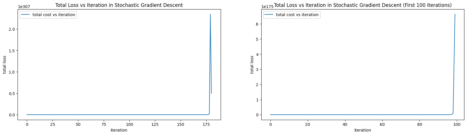
The same experiments with gradient descent show that SGD can be sensitive to changes in stepsizes in ways that gradient descent is not.
Not covered here: a step-by-step discussion of the SGD runs for each step size.
Solution: Part I, Question 7
Why would your choice of initial parameters matter? Let’s recall our visualization of the objective function:
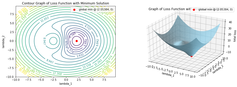
We see, from the above graphs, that our total loss function has three stationary points (points in the parameter space where the gradient of the total loss function is zero):
local and global minimum at approximately (2.05384, 0), with total loss -9.9341
local maximum at approximately (-2.47865, 0), with total loss 11.9546
saddle point at approximately (-5.36325, 0), with total loss 8.16153
At each of these points, since the gradient is very nearly zero, we’d expect gradient descent to be stationary (the algorithm will not make any updates to the parameters, since updates are proportional to the gradient vector). Thus, if gradient descent lands on either the local max or the saddle point during its path through the parameter space then it will not converge on the correct optimal value.
But how often can gradient descent get stuck at the local max or the saddle point? Since in every step of gradient descent, we update the parameter to decrease total loss, it is very unlikely that we will end up at the local max (if our initialization is not at the local max). On the other hand, if we are initialized on the left of the local max and along the straight line passing through the local max and the saddle point, then we are nearly guaranteed to land in the saddle point. The intuition is: if you initialize on the right side of the hill containing our local max, then we will “slide down” right into the global min, but if we initialize on the left side of the hill, then we will “slide down” into the saddle point.
Let’s experiment with several initializations for gradient descent.
fig, ax = plt.subplots(2, 4, figsize=(25, 10))

lambdas_inits = [[-2.47865, 0], [-3, 0], [-5, 0], [-10, 0]]

for i in range(len(lambdas_inits)):
    history, _ = gradient_descent(x, y, lambdas_inits[i], step_size=10., maxsteps=100000)
    history = np.array(history)
    costs = L(history[:, 0], history[:, 1], x, y)
    ax[0, i].plot(range(len(costs)), costs, label='total cost vs iteration')
    ax[0, i].set_xlabel('iteration')
    ax[0, i].set_ylabel('total cost')
    ax[0, i].set_title('Total Cost vs Iteration in Gradient Descent,\n init @({}, 0), stepsize 10\n'.format(lambdas_inits[i][0]))
    ax[0, i].legend(loc='best')

    ax[1, i].plot(range(len(costs[:500])), costs[:500], label='total cost vs iteration')
    ax[1, i].set_xlabel('iteration')
    ax[1, i].set_ylabel('total cost')
    ax[1, i].set_title('Total Cost vs Iteration in Gradient Descent,\n initial 500 iterations, \n init @({}, 0), stepsize 10\n'.format(lambdas_inits[i][0]))
    ax[1, i].legend(loc='best')

plt.tight_layout()
plt.show()
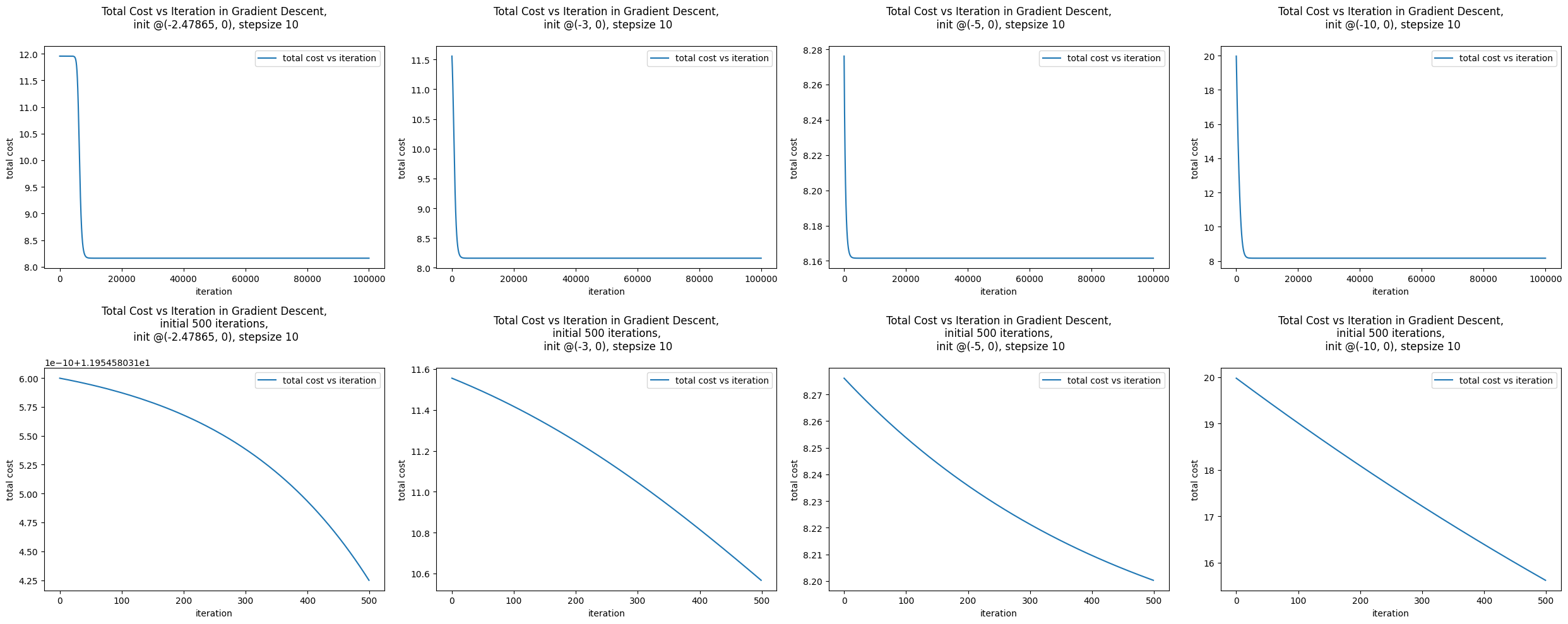
We see that in each case, for each initial choice of lambdas, gradient descent proceeded towards the saddle point and, once having reached the saddle, remained at the saddle.
What is unexpected is the behaviour of gradient descent for the initialization (-2.47865, 0). Recall that at \((\lambda_1, \lambda_2) = (-2.47865, 0)\), the total loss function has a local max and at a local max the gradient is zero. So why doesn’t gradient descent get stuck at the local max? Well, it did, for about a couple of thousands of iterations (see left-most column of graphs above). But recall that we are approximating the location of the local max with \((-2.47865, 0)\), thus the gradient at \((-2.47865, 0)\) is close to zero but not exactly zero. This means that your gradient descent algorithm maybe making microscopic progress in the parameter space and that if you let it run for long enough, it might move to a region of the space where the gradients are large again. Note that, in practice, we never let gradient descent algorithms crawl! That is, we terminate the algorithm whenever it ceases to make “large” updates to the parameters. This is because for a general complex objective function there is not always a way for us to predict how long the algorithm must run before it gets “unstuck” or converges on an acceptable solution.
print('gradient at approximate local max (-2.47865, 0):', grad(-2.47865, 0, x, y))
print('gradient at approximate saddle (-5.36325, 0):', grad(-5.36325, 0, x, y))
gradient at approximate local max (-2.47865, 0): [1.27466626e-05 0.00000000e+00]
gradient at approximate saddle (-5.36325, 0): [-1.27991562e-06  0.00000000e+00]
So how will stochastic gradient descent behave around stationary points (points at which the gradient of the total loss function is zero)? Recall that stochastic gradient descent does not compute the gradient of the “real” objective function in each iteration. Rather it computes an “approximate” gradient using just one data point (i.e. it compute the gradient of the loss function at just one random point).
Earlier in this chapter we saw how this descent with “approximate” gradients can be less efficient - while gradient descent beelines for the optimal solution, stochastic gradient descent can meander in the parameter space. However, the same “noisy” trajectories stochastic gradient descent can also help us avoid getting stuck in non-optimal stationary points. The intuition is simple, at places where the total loss function has zero gradient, it is possible that a random “approximate” loss function will not have zero gradient.
Let’s experiment with stochastic gradient descent for the same set of initializations in the parameter space:
fig, ax = plt.subplots(1, 4, figsize=(20, 4))

lambdas_inits = [[-2.47865, 0], [-3, 0], [-5, 0], [-10, 0]]

for i in range(len(lambdas_inits)):
    history, epoch, _ = sgd(x, y, lambdas_inits[i], init_shuffle=True, step_size=10., max_epochs=8, output=False)
    history = np.array(history)
    costs = L(history[:, 0], history[:, 1], x, y)
    print('Final cost with initialization @ ({}, {}) in {} epochs is {}'.format(lambdas_inits[i][0], lambdas_inits[i][1], epoch, costs[-1]))
    ax[i].plot(range(len(costs)), costs, label='total cost vs iteration')
    ax[i].set_xlabel('iteration')
    ax[i].set_ylabel('total cost')
    ax[i].set_title('Total Cost vs Iteration in Stochastic Gradient Descent,\n init @({}, 0), stepsize 10\n'.format(lambdas_inits[i][0]))
    ax[i].legend(loc='best')

plt.tight_layout()
plt.show()
Final cost with initialization @ (-2.47865, 0) in 8 epochs is 11.954580308623719
Final cost with initialization @ (-3, 0) in 8 epochs is 8.161528699372983
Final cost with initialization @ (-5, 0) in 8 epochs is 8.161528699372983
Final cost with initialization @ (-10, 0) in 8 epochs is 8.161528699372983

We see that with step size 10, stochastic gradient descent appears to do no better than gradient descent in escaping stationary points! So is our intuition about stochastic descent wrong? Well, recall that stochastic descent is very sensitive to stepsize, in particular, the “stochastic-ness” (or randomness) of the algorithm can be either amplified or diminished by the step-size. Choose sufficiently small step sizes, you may not see too much randomness in the behaviour of your SGD; choose sufficiently large step sizes, you may observe very unexpected results.
Let’s increase the step size to 50 and see what happens:
fig, ax = plt.subplots(1, 4, figsize=(20, 4))

lambdas_inits = [[-2.47865, 0], [-3, 0], [-5, 0], [-10, 0]]

for i in range(len(lambdas_inits)):
    history, epoch, _ = sgd(x, y, lambdas_inits[i], init_shuffle=True, step_size=50, max_epochs=8, output=False)
    history = np.array(history)
    costs = L(history[:, 0], history[:, 1], x, y)
    print('Final cost with initialization @ ({}, {}) in {} epochs is {}'.format(lambdas_inits[i][0], lambdas_inits[i][1], epoch, costs[-1]))
    ax[i].plot(range(len(costs)), costs, label='total cost vs iteration')
    ax[i].set_xlabel('iteration')
    ax[i].set_ylabel('total cost')
    ax[i].set_title('Total Cost vs Iteration in Stochastic Gradient Descent,\n init @({}, 0), stepsize 50\n'.format(lambdas_inits[i][0]))
    ax[i].legend(loc='best')

plt.tight_layout()
plt.show()
Final cost with initialization @ (-2.47865, 0) in 1 epochs is -9.934103951511823
Final cost with initialization @ (-3, 0) in 2 epochs is -9.934103767700416
Final cost with initialization @ (-5, 0) in 2 epochs is -9.934103785311704
Final cost with initialization @ (-10, 0) in 0 epochs is -9.934103619663786

So in this case, we see that SGD is able to converge onto the correct optimum for all initial values of lambdas we chose! With an increase in the step size, we were able to amplify the randomness of the algorithm enough to help us escape stationary points!
Now, this begs the question:
What step size should I choose to help SGD escape undesirable stationary points?
For example, is it true that the bigger the step-size the faster my SGD algorithm converges onto the global minimum? Let’s run SGD on the same set of initial lambda values again, this time, with step size 500.
fig, ax = plt.subplots(1, 4, figsize=(20, 4))

lambdas_inits = [[-2.47865, 0], [-3, 0], [-5, 0], [-10, 0]]

for i in range(len(lambdas_inits)):
    history, epoch, _ = sgd(x, y, lambdas_inits[i], init_shuffle=True, step_size=500, max_epochs=8, output=False)
    history = np.array(history)
    costs = L(history[:, 0], history[:, 1], x, y)
    print('Final cost with initialization @ ({}, {}) in {} epochs is {}'.format(lambdas_inits[i][0], lambdas_inits[i][1], epoch, costs[-1]))
    ax[i].plot(range(len(costs)), costs, label='total cost vs iteration')
    ax[i].set_xlabel('iteration')
    ax[i].set_ylabel('total cost')
    ax[i].set_title('Total Cost vs Iteration in Stochastic Gradient Descent,\n init @({}, 0), stepsize 500\n'.format(lambdas_inits[i][0]))
    ax[i].legend(loc='best')

plt.tight_layout()
plt.show()
Final cost with initialization @ (-2.47865, 0) in 0 epochs is inf
Final cost with initialization @ (-3, 0) in 0 epochs is inf
Final cost with initialization @ (-5, 0) in 0 epochs is inf
Final cost with initialization @ (-10, 0) in 0 epochs is inf

Just as we saw before, when the step size is “large”, stochastic gradient descent can have unexpected and deeply undesirable behaviours (for contrast, run gradient descent using a stepsize of 500).
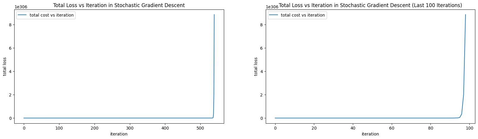
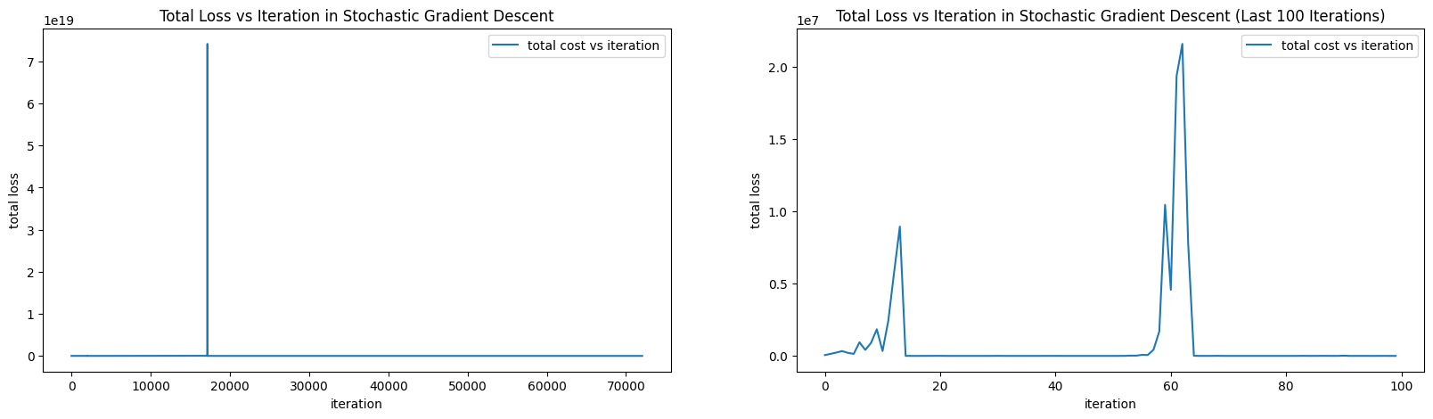
Lesson Learned: Unlike gradient descent, which can get stuck in undesirable stationary points, the randomness of stochastic gradient descent can keep the algorithm moving towards the global optimum. But this benefit can only be realized by the correct choice of step size, for a choice of step size that is too small, the randomness of SGD (with fixed step size) is insufficient to move it out of a stationary point; for a choice of step size that is too large, the randomness of SGD (with fixed step size) may prevent the algorithm from converging or even getting close to the global optimum.
Not covered here: gradient descent with a learning rate of 50.
Exercise: Part II: Broader Impact Analysis
Starting in 2020, major machine learning conferences are beginning to ask authors as well as reviewers to explicitly consider the broader impact of new machine learning methods. To properly evaluate the potential good or harm that a piece of technology (AI or not) can do to the general public, we need to be aware that no technology is deployed in ideal conditions or in perfectly neutral contexts. In order to assess the potential broader impact of technology, we need to analyze the social systems/institutions of which these technologies will become a part.
To help you analyze the broader impact of your technology, begin by considering the following questions:
I. Identify the relevant socio-technical systems
In what social, political, economic system could the tech be deployed?
How would the tech be used in these systems (what role will it take in the decision making processes)?
II. Identify the stakeholders
Who are the users?
Who are the affected communities (are these the users)?
Hint: users are typically decision makers who will use the technology as decision aids (e.g. doctors), whereas affected communities may be folks who are impacted by these decisions but who are not represented in the decision making process (e.g. patients).
III. What types of harm can this tech do?
What kinds of failures can this tech have?
What kinds of direct harm can these failures cause?
What kinds of harm can the socio-technical system cause?
Hint: many technical innovations have niche applications, they may sit in a long chain of decision making in a complex system. As such, it may seem, at first glance, that these technologies have no immediate real-life impact. In these cases, it’s helpful to think about the impact of the entire system and then think about how the proposed innovations aid, hamper or change the goals or outcomes of this system.
IV. What types of good can this tech do?
What kinds of needs do these users/communities have?
What kinds of constraints do these users/communities have?
(Impact) Analyze the broader impact of this pricing model. Focus on anticipating ways these models can interact with other components of the decision systems in which they will be deployed, identifying end-users, affected communities as well as anticipating the effects (positive and negative) on affected communities (in particular, does the model have the same effect on all subpopulations in the affected communities?).
Hint: the objective function we are minimizing here is the construction cost, who benefits from minimizing the this objective function, whose utility function might be in tension with this objective function?
How do the quirks and artifacts of the optimization algorithm impact the end-user (i.e. how is your end-user affected by the optimization procedure and the hyperparameters you choose)? How do your design choices in optimization impact the affected community?
16.8. Further Reading#
Simulated Annealing and Non-Convex Optimization