Bayesian Modeling

3. Bayesian Modeling#

This chapter is adapted from AM207 (Harvard, Fall 2021). Watch the recorded lecture.

In this chapter

Review of the Method of Maximum Likelihood
Models for Real Data
The Beta-Binomial Model
Bayesian Modeling
Connections and Comparisons with Frequentist Inference

3.1. Review of the Method of Maximum Likelihood#

The Method of Maximum Likelihood#

(Model) Assume observations from $N$ number of independently and identically distributed outcomes, $Y_1, \ldots, Y_N$, with $Y_n \sim p(Y|\theta)$ and where $\theta$ is the set of parameters of the distribution $p(Y|\theta)$. The likelihood function is

\[\begin{aligned} \mathcal{L}(\theta) = \prod_{n=1}^N p(y_n | \theta) \end{aligned}\]
(Inference) We estimate $\theta$ using the maximum likelihood estimate, defined as

\[\begin{aligned} \theta_{\text{MLE}} = \underset{\theta}{\mathrm{argmax}}\; \mathcal{L}(\theta) = \underset{\theta}{\mathrm{argmax}}\; \prod_{n=1}^N p(y_n | \theta) \end{aligned}\]
(Inference Method)
- Unconstrained Optimization: if $\theta$ doesn’t need to satisfy any special property, then it’s as simple as setting the gradient of the likelihood equal to zero and solving! (Except it’s not that simple!)
- Constrained Optimization: if $\theta$ needs to satisfy special properties, then it’s as simple as setting the gradient of the Lagrangian of the likelihood and the constraint equal to zero and solving! (Except it’s not that simple!)

Evaluating the MLE#

If we have the true parameters $\theta$, we can compute the Mean Squared Error:

\[ \mathrm{MSE}_{\theta} = \mathbb{E}_{Y^{\theta}}\left[(\theta_{\text{MLE}}\left(Y^\theta\right) - \theta)^2\right] \]

If we don’t have the true parameters $\theta$, we can use $\theta_{\text{MLE}}$ predict or simulate data and compare it with the observed data, i.e. sample

\[ Y^{\theta_{\text{MLE}}} \sim p(Y| \theta_{\text{MLE}}), \]

compare $Y^{\theta_{\text{MLE}}}$ and $Y^{\theta}$.

Properties of The Maximum Likelihood Estimator#

Why Choose MLE? Asymptotically, i.e. given an infinite number of samples, the MLE is

Consistent: $\theta_{\text{MLE}}$ approaches the true parameters $\theta$.
Unbiased: The average $\theta_{\text{MLE}}$, taken over many different samples of the data, is $\theta$.
Minimum Variance: The MLE has the lowest variance of all unbiased estimators.

Why Not Choose MLE? When the sample size is “small”, the MLE can be

Overfitted: The MLE can is sensitive to outliers in the data.
Biased: The average $\theta_{\text{MLE}}$, taken over many different data samples, is not $\theta$.
Imprecise: The MLE can have high variance.

What Other Estimators are There?

Method of Moments
Minimum Variance Unbiased Estimator
Regularized MLE

Note: the computation of (1) and (2) can be much more complex than MLE.

Is Bias Always Bad?#

Recall that we can use the properties of expectations to decompose the mean squared error of the maximum likelihood estimator:

\[ \mathrm{MSE}_{\theta_{\text{MLE}}} = \underbrace{\mathbb{E}\left[(\theta_{\text{MLE}} - \mathbb{E}[\theta_{\text{MLE}}])^2\right]}_{\text{variance}} + \underbrace{\left( \mathbb{E}[\theta_{\text{MLE}}] - \theta\right)^2}_{\text{bias}} \]

Although we want an unbiased estimator, the above decomposition says that if the variance of the estimator is high our expected error will nonetheless be high.

The variance-bias trade-off refers to the phenomenon that, in many cases, when estimators have low bias they have high corresponding variance (and vice versa), and hence high MSE.

Going deeper: Decomposition of MSE

\[\begin{split}\begin{aligned} \mathrm{MSE}_{\theta_{\text{MLE}}} &= \mathbb{E}_{Y^\theta} \left[\left(\theta_{\text{MLE}} - \theta \right)^2 \right]\\ &= \mathbb{E}_{Y^\theta}\left[\left( \theta_{\text{MLE}} - \mathbb{E}[\theta_{\text{MLE}}] + \mathbb{E}[\theta_{\text{MLE}}] - \theta \right)^2 \right]\\ &= \mathbb{E}\left[\left(\theta_{\text{MLE}} - \mathbb{E}[\theta_{\text{MLE}}]\right)^2\right] + \mathbb{E}\left[\left(\mathbb{E}[\theta_{\text{MLE}}] - \theta \right)^2 \right] + 2\mathbb{E}\left[ (\theta_{\text{MLE}} - \mathbb{E}[\theta_{\text{MLE}}])(\mathbb{E}[\theta_{\text{MLE}}] - \theta)\right]\\ &= \underbrace{\mathbb{E}\left[(\theta_{\text{MLE}} - \mathbb{E}[\theta_{\text{MLE}}])^2\right]}_{\text{variance}} + \underbrace{\left( \mathbb{E}[\theta_{\text{MLE}}] - \theta\right)^2}_{\text{bias}} \end{aligned}\end{split}\]

Example of the Bias Variance Trade-off Let $Y \sim\mathcal{N}(0, \sigma^2)$. Consider two estimators of the variance $\sigma^2$:

$\widehat{\theta}_1(Y) = Y^2$
$\widehat{\theta}_2(Y) = \frac{1}{3}Y^2$

The expected values of the estimators are:

$\mathbb{E}[\widehat{\theta}_1] = \mathbb{E}[Y^2]=\sigma^2$, using the fact $Y^2$ is a Gamma distribution with mean $\sigma^2$.
$\mathbb{E}[\widehat{\theta}_1] = \mathbb{E}[Y^2]=\frac{1}{3}\sigma^2$ So we see that $\widehat{\theta}_1$ is unbiased, whereas $\widehat{\theta}_2$ is biased.

Note that the two estimators are both of the form $cY^2$ where $c$ is a constant. We can compute the MSE, in a general way, for this class of estimators:

\[\begin{split}\begin{aligned} \mathrm{MSE}_{\widehat{\theta}} &= \mathbb{E}\left[\left(\widehat{\theta}_2 - \sigma^2\right)^2\right]\\ &= \mathbb{E}\left[c^2Y^4 - 2\sigma^2 cY^2 + \sigma^4 \right]\\ &= c^2\mathbb{E} \left[Y^4 \right] - 2\sigma^2c\mathbb{E} \left[Y^2 \right] + \sigma^4\\ &= 3c^2\sigma^4 - 2c\sigma^4 + \sigma^4\\ &= \sigma^4(3c^2 - 2c + 1) \end{aligned}\end{split}\]

From the expression of the MSE, we can find the $c$ that will minimize $\mathrm{MSE}_{\widehat{\theta}}$ - this involves finding the stationary points of the derivative of $\mathrm{MSE}_{\widehat{\theta}}$ (and then checking concavity/convexity!):

\[ \frac{d}{dc}\mathrm{MSE}_{\widehat{\theta}} = \sigma^4(6a - 2) = 0 \]

We see that $\mathrm{MSE}_{\widehat{\theta}}$ has a unique global minimum at $c = \frac{1}{3}$. That is, the biased estimator $\widehat{\theta}_2$ has smaller MSE than the unbiased estimator $\widehat{\theta}_1$.

Limitations of MLE: Overfitting Under Scarcity of Data#

Suppose that we have three observations from a Bernoulli distribution, $Ber(\theta)$: $\{ H, H, H\}$. From what we’ve see before, the MLE of $\theta$ is

\[ \theta_{\text{MLE}} = \frac{3}{3} = 1. \]

Is this a good estimate of the bias of the coin? What can we do to make this estimate better?

Suppose that we have two YouTube videos with 4/5 likes and 3,500/5,000 likes respectively. We can model the probability that a viewer will like each video as two Bernoulli distributions, $Ber(\theta_1)$, $Ber(\theta_2)$, where $\theta_i$ is the “inherent” likeability of each video.

Again, we can compute the MLE of the Bernoulli parameters:

\[ \theta_1 = 4/5 = 0.8,\; \theta_2 = 3,500/5,000 = 0.75. \]

It is fair to say that the second video is more likeable base on our estimates?

Regularization#

We can prevent MLE from overfitting to the observations when training data is scarce by constraining it from unreasonable values.

Recall that in order to prevent the MLE solution for linear regression from learn unrealistically large slopes and intercepts, we add $\ell_2$-regularization on the model parameters during training, essentially forcing the parameters to stay as small (close to zero) as they can be while still capturing the data.

Similarly, if want the MLE of the parameter $\theta$ of a Bernoulli distribution to avoid extreme values (1 and 0), we need to ‘anchor’ our estimation of $\theta$ to some ‘reasonable’ value:

\[\begin{aligned} \theta_{\text{MLE Reg.}} = \frac{\text{# positive outcome} + \alpha}{\text{# total trials} + \beta} \end{aligned}\]

The fraction $\alpha/\beta$ expresses your notion of what is a reasonable looking probability.

But is regularization a principled way to perform inference (i.e. will it ruin the nice properties of MLE)? How do you choose the hyperparameters $\alpha$, $\beta$ in a principled manner?

3.2. Models for Real Data#

Going deeper: Die Roll

We can model the outcome, $Y$, of a single dice roll with a categorical distribution,

\[ Y \sim Cat(\theta) \]

where $\theta = [\theta_1 \ldots \theta_6]$ is a vector satisfying $\sum_{i=1}^6 \theta_i = 1$, and where $\theta_i$ is the probability of rolling a number $i$.

Given $Y_1,\ldots, Y_N$ identically and independently distributed outcomes with $Y_n \sim Cat(\theta)$. Denote the total number observed for each face as a vector $F = [f_1 \ldots f_6]$, where $f_i$ is the number of times the number $i$ was rolled. Then $F$ can be modeled with a multinomial distribution,

\[ F \sim Mul(N, \theta). \]

Model Critique: What are the assumptions made in this model? Are they realistic?

Video Ranking#

We can model the outcome, $Y$, of a user rating for a specific YouTube video as a Bernoulli distribution,

\[ Y \sim Ber(\theta) \]

where $\theta$ is the probability that a user will like the video.

Given $Y_1,\ldots, Y_N$ identically and independently distributed outcomes with $Y_n \sim Ber(\theta)$. Denote the total number of likes by $L$. Then $L$ can be modeled with a binomial distribution,

\[ L \sim Bin(N, \theta). \]

Model Critique: What are the assumptions made in this model? Are they realistic?

Kidney Cancer Rates#

Given a dataset with $N$ number of US counties and the incidents of kidney cancer in each county, we can model the observed incidents of cancer, $C_n$, of the $n$-th county with a Poisson distribution,

\[ C_n \sim Poi(T_n\theta_n) \]

where $T_n$ is the total population of the county and $\theta_n$ is the “true” cancer rate of the county.

Model Critique: What are the assumptions made in this model? Are they realistic?

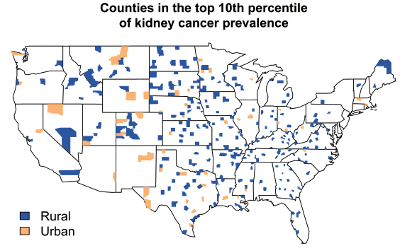
The following is a visualization of the counties with the highest rates of kidney cancer (Gelman 1998). Is there any noticeable spatial pattern in these maps? Recall that the MLE of the rate of the Poisson distribution for each county is $\frac{C_n}{T_n}$.

Birth Weights#

In our lab, we work with IVF clinics to build models for prediction and data analysis. One of our current tasks is to model the birth weights of the infants born in the clinic.

Naively, given observed birth weights $Y_1, \ldots, Y_N$, we can model each outcome $Y_n$ with a normal distribution,

\[ Y_n \sim \mathcal{N}(\mu, \sigma^2) \]

where $\mu$ is the average birth weight for this population and $\sigma^2$ is the population variance.

Model Critique: What are the assumptions made in this model? Are they realistic?

3.3. The Beta-Binomial Model#

The Coin Toss Model: Revisited#

Suppose that we have three observations from a Bernoulli distribution, $Ber(\theta)$: $\{ H, H, H\}$. The MLE of $\theta$ is

\[ \theta_{\text{MLE}} = \frac{3}{3} = 1. \]

This is a clear case of the MLE overfitting to the observed data.

Last time, you’d suggested tying the estimate to some fixed reasonable number, for example,

\[ \theta_{\text{MLE Reg}} = \frac{H + 1}{N + 2}, \]

and in general,

\[ \theta_{\text{MLE Reg}} = \frac{H + \alpha}{N + \beta}. \]

The terms $\alpha$ and $\beta$ are called regularization terms .

Question: What is the effect of $\alpha$, $\beta$ on our estimate? What values should we choose for $\alpha$, $\beta$?

Incorporating Prior Beliefs#

Our choice of the regularization terms, $\alpha$, $\beta$, depends on our prior beliefs about the coin. The way we chose to incorporate these beliefs doesn’t indicate any uncertainty.

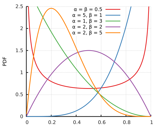
Alternatively, we can incorporate our prior belief about $\theta$ as a distribution, this is called the prior distribution. Since $\theta$ is a number between 0 and 1, a beta distribution is an appropriate choice.

The Beta-Binomial Model#

A model that involves both a likelihood for the data and prior on the parameters in the likelihood is called a Bayesian model.

Bayesian Model for Coin Flip

\[\begin{split}\begin{aligned} Y &\sim Bin(N, \theta),\quad &\text{(Likelihood)}\\ \theta &\sim Beta(\alpha, \beta),\quad &\text{(Prior)} \end{aligned}\end{split}\]

where $\alpha, \beta$ are called hyperparameters of the model.

Now, computing the MLE no longer makes sense (since the MLE only considers the likelihood). Luckily, Bayes’ Rule allows us to derive a distribution that considers both the prior and the likelihood:

\[\begin{aligned} p(\theta | Y) = \frac{\overbrace{p(Y| \theta)}^{\text{likelihood}} \overbrace{p(\theta)}^{\text{prior}}}{\underbrace{p(Y)}_{\text{marginal data likelihood}}} = \frac{p(Y, \theta)}{\int p(Y, \theta) d\theta} \end{aligned}\]

The distribution $p(\theta | Y)$ is called the posterior.

Posterior for the Beta-Binomial Model#

In our case, the posterior is given by

\[\begin{aligned} p(\theta | Y) = \frac{p(Y| \theta)p(\theta)}{p(Y)} = \frac{\overbrace{{N \choose Y}\theta^{Y}(1- \theta)^{N-Y}}^{\text{binomial pdf}} \overbrace{\frac{1}{B(\alpha, \beta)} \theta^{\alpha - 1} (1 - \theta)^{\beta - 1}}^{\text{beta pdf}}}{p(Y)} \end{aligned}\]

We can rewrite the posterior as

\[\begin{aligned} p(\theta | Y) = const * \theta^{(Y+\alpha) - 1}(1 - \theta)^{(N-Y + \beta) - 1} \end{aligned}\]

where $const = \frac{{N \choose Y}}{B(\alpha, \beta)p(Y)}$ must be the normalizing constant for $p(\theta | Y)$.

We recognize the posterior as a beta distribution, $Beta(Y+\alpha, N-Y + \beta)$! Can you see why?

Interpreting the Posterior: Bayesian Update#

Rather than a point estimate for $\theta$, we now have a posterior distribution, $p(\theta|Y)$, over $\theta$. What does the posterior tell us about $\theta$?

Since the prior distribution $p(\theta)$ encoded our beliefs about $\theta$ along with our uncertainty, it is natural to interpret the posterior as yet another belief about $\theta$.

Since the posterior includes the likelihood, this belief has been updated by the data.

Simulation: Bayesian Update for the Coin Flip#

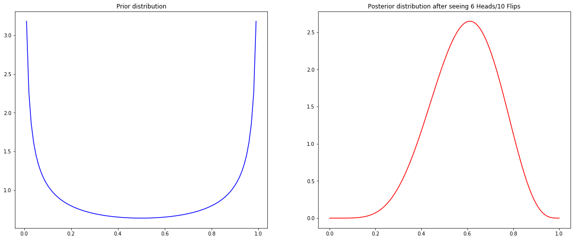
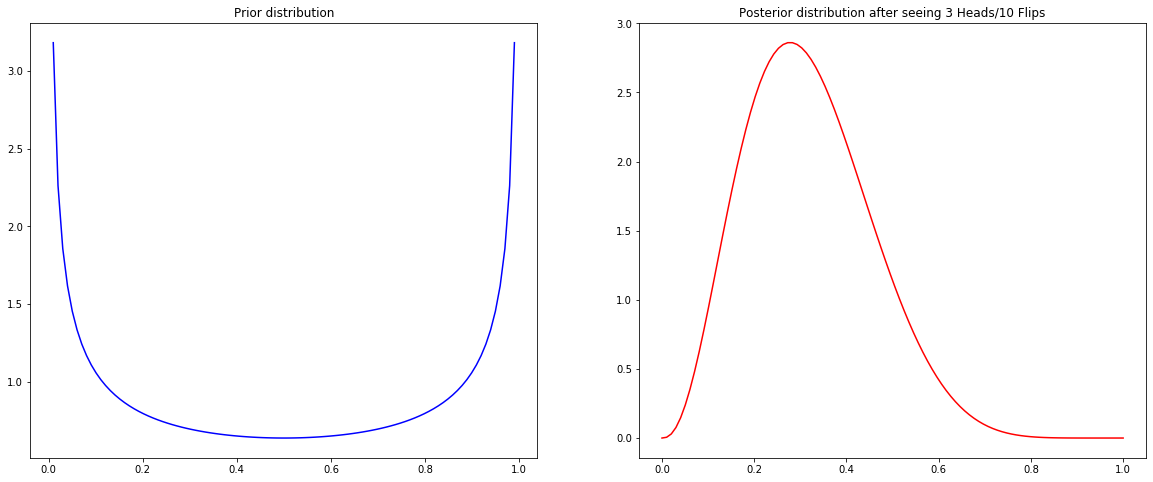
What is the effect of the choice of the prior on the posterior? What is the effect of the number of observations, $N$, on the posterior?

fig, ax = plt.subplots(1, 2, figsize=(20, 8))
ax = plot_prior_posterior(ax, prior, posterior, H, N)
plt.show()

../_images/e4c579eb58b4d1bb45743f5a9f6076bd4e3be6fcfa1845d5945a0c36f4ebe7a1.png

../_images/4feac302b92737fc3480ce39fc145c47b47f395c5e8d05637aaa283ab71b73a4.png

Making Predictions#

If the posteriors we infer represent beliefs, how do we evaluate these beliefs?

In the case that we the true parameter $\theta^{\text{true}}$, we can check to see if the posterior assigns high likelihood to $\theta^{\text{true}}$, and the certainty the posterior has around $\theta^{\text{true}}$.
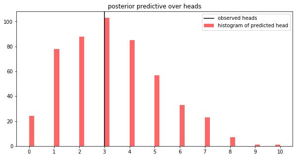
When we do not know $\theta^{\text{true}}$, we can simulate data $Y^{\theta}$ using samples of $\theta$ from the posterior. We compare the distribution of simulated data, or posterior predictive, to the observed data.

Simulation: Posterior Predictive for the Coin Flip#

posterior_samples = np.random.beta(posterior_alpha, posterior_beta, size=500)
posterior_pred = [np.random.binomial(N, theta_sample, 1)[0] for theta_sample in posterior_samples]

fig, ax = plt.subplots(1, 1, figsize=(10, 5))
ax = plot_posterior_predictive(ax, posterior_pred, H)
plt.show()

../_images/eab37958b30bb544941cdd3038d957a2f151793def563369995a85e61e680122.png

3.4. Bayesian Modeling - A Summary#

The Bayesian Modeling Process#

In order to make statements about $Y$, the outcome, and $\theta$, parameters of the distribution generating the data, we form the joint distribution over both variables and use the various marginals/conditional distributions to reason about $Y$ and $\theta$.

we form the joint distribution over both variables $p(Y, \theta) = p(Y | \theta) p(\theta)$.
we can condition on the observed outcome to make inferences about $\theta$,

\[ p(\theta | Y) = \frac{p(Y, \theta)}{p(Y)} \]

where $p(\theta | Y)$ is called the posterior distribution and $p(Y)$ is called the evidence.
before any data is observed, we can simulate data by using our prior

\[ p(Y^*) = \int_\Theta p(Y^*, \theta) d\theta = \int_\Theta p(Y^* | \theta) p(\theta) d\theta \]

where $Y^*$ represents new data and $p(Y^*)$ is called the prior predictive.
after observing data, we can simulate new data similar to the observed data by using our posterior

\[ p(Y^*|Y) = \int_\Theta p(Y^*, \theta|Y) d\theta = \int_\Theta p(Y^* | \theta) p(\theta | Y) d\theta \]

where $Y^*$ represents new data and $p(Y^*|Y)$ is called the posterior predictive.

Evaluating Bayesian Models#

As we have seen in the Beta-Binomial model, we can simulate the posterior (and prior) predictive rather than compute them analytically. That is, you don’t need to know the pdf of $p(Y^*|Y)$.

The posterior predictive can be represented by samples of predictions:

we sample values of $\theta_n$ from the posterior, $p(\theta|Y)$.
we sample an outcome $Y_n$ from $p(Y|\theta_n)$ for each posterior sample $\theta_n$.

The set $Y_n$ we obtain empirically represents the posterior predictive distribution $p(Y^*|Y)$.

Going deeper: Aside

How do we evaluate the quality of our Bayesian model: how appropriate was our choice of prior? How appropriate was our choice of noise structure for the data (i.e. how appropriate is our choice of likelihood)?

Evaluating Bayesian models is challenging for two reasons:

Instead of learning a single best estimate of the model parameters $\theta$, like in the case of maximum likelihood estimation, we learn a distribution over possible values of $\theta$, $p(\theta|Y)$
In real life we do not have access to the ground truth values of model parameters

Thus, we evaluate our model by seeing how well it fits the observed data. That is, we check to see how well our predicted distribution of $Y^*$, $p(Y^* | Y)$, matches up with the observed data $Y^*$.

When we are able to visualize the data (i.e. when $Y^*$ is low-dimensional), we can visualize both data $Y^*$ and samples from $p(Y^* | Y)$. If the model is a good fit for the data, these two plots should be similar.

But what if it’s not possible to visualize the data?

Where do Priors Come From?#

Hopefully you’ve noticed a key property of the priors we chose:

All the priors combined with the likelihood to form a distribution we recognize! Specifically, the posterior distribution is of the same type as the prior!

These priors are called conjugate priors for the corresponding likelihoods. This is a purely mathematical property.

Question: is it right to choose priors that are mathematically convenient? What is a good way to choose a prior? What if we “choose wrong”?

Going deeper: Uninformative Priors: How to Say I Don’t Know

If you don’t have a strong prior believe about the parameters in the likelihood, you should choose a prior that has no effect when combined with the likelihood – i.e. let the data speak for itself.

Example: In the Beta-Binomial model, is there a choice of the hyperparameters of the prior that has no effect on the posterior?

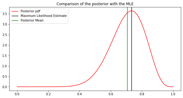
We might try $Beta(1, 1)$, which is the uniform distribution over $[0, 1]$. The posterior $p(\theta|Y)$ is then $Beta(Y + 1, N - Y + 1)$. In the following example, visualizing the posterior, we see that the posterior assigns the highest mass to the MLE of $\theta$. But the posterior assigns more mass to values of $\theta$ smaller than the MLE. In this sense, the prior does inform the posterior.

../_images/3d645d6e5d4d3c49e13ab7ea3e41bb6c1c1949d33f5b8ac10514d67a32950f0c.png

Going deeper: Aside

There is a general purpose technique for creating non-informative priors, called Jeffreys priors, which places less prior weight on parameter values where the likelihood function is flat. This prevents the prior from having undue influence on the posterior.

There are many resources that cover the construction of Jeffreys priors for common likelihoods.

3.5. Summary#

How do we evaluate the fit of our MLE model?
- With regression it’s easy, you plug $x_n$ into $f_{\theta_\text{MLE}}(x)$ and then compare the prediction $\widehat{y}_n$ with $y$. But what if we don’t have any inputs, $x_n$, what if we just have $y_n$? In this case we would not be able to predict a $\widehat{y}_n$ for a specific $y_n$.
What are the potential drawbacks of MLE (in particular, under data scarcity)?
- What are some common fixes for the drawbacks of MLE?
- What are some potential issues with these fixes?
What is the point of adding priors to our models? Specifically how does adding priors to our model mitigate some of the drawbacks of MLE?
How should we interpret the posterior of a Bayesian model and why?
What is a posterior predictive? What is the relationship between the posterior predictive and the posterior? What is the point of deriving the posterior predictive (i.e. once we derive the posterior isn’t that enough)?
How do we evaluate a Bayesian model (the posterior is a distribution over plausible models not a single “best” model)?
How do we choose priors for Bayesian models? What if we chose wrong? Why did we choose a Beta prior for the binomial model for the coin flip data?

3.6. Exercises#

These problems were originally assigned as homework. Data files are in the book’s data/ folder. Worked solutions, where available, are collapsed beneath the questions they answer; try each problem before expanding them.

Problem Set: Review of Statistical Modeling and Scientific Computing#

Problem Description#

In the competitive rubber chicken retail market, the success of a company is built on satisfying the exacting standards of a consumer base with refined and discriminating taste. In particular, customer product reviews are all important. But how should we judge the quality of a product based on customer reviews?

On Amazon, the first customer review statistic displayed for a product is the average rating. The following are the main product pages for two competing rubber chicken products, manufactured by Lotus World and Toysmith respectively:

Lotus World	Toysmith

Clicking on the ‘customer review’ link on the product pages takes us to a detailed break-down of the reviews. In particular, we can now see the number of times a product is rated a given rating (between 1 and 5 stars).

Lotus World	Toysmith

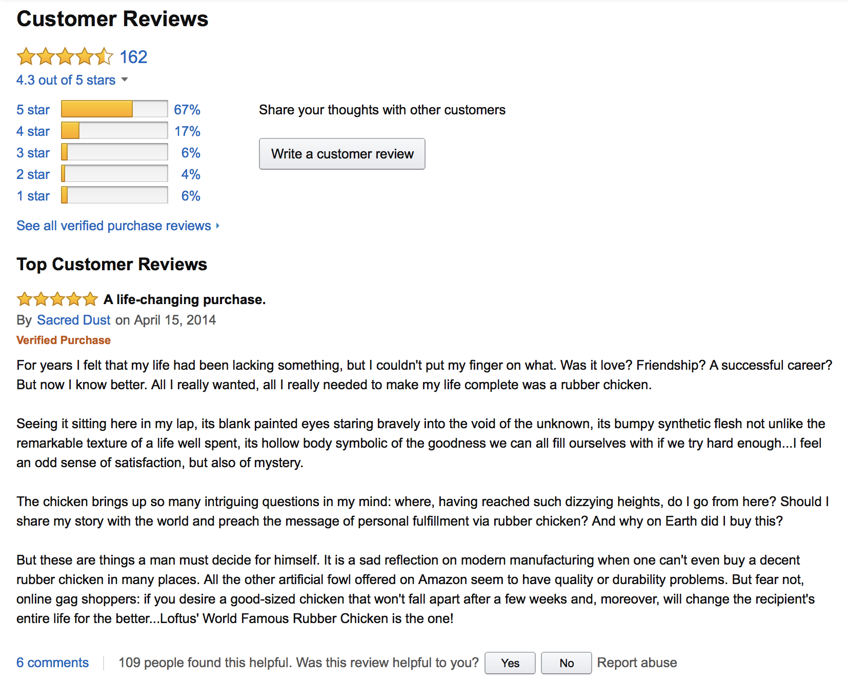
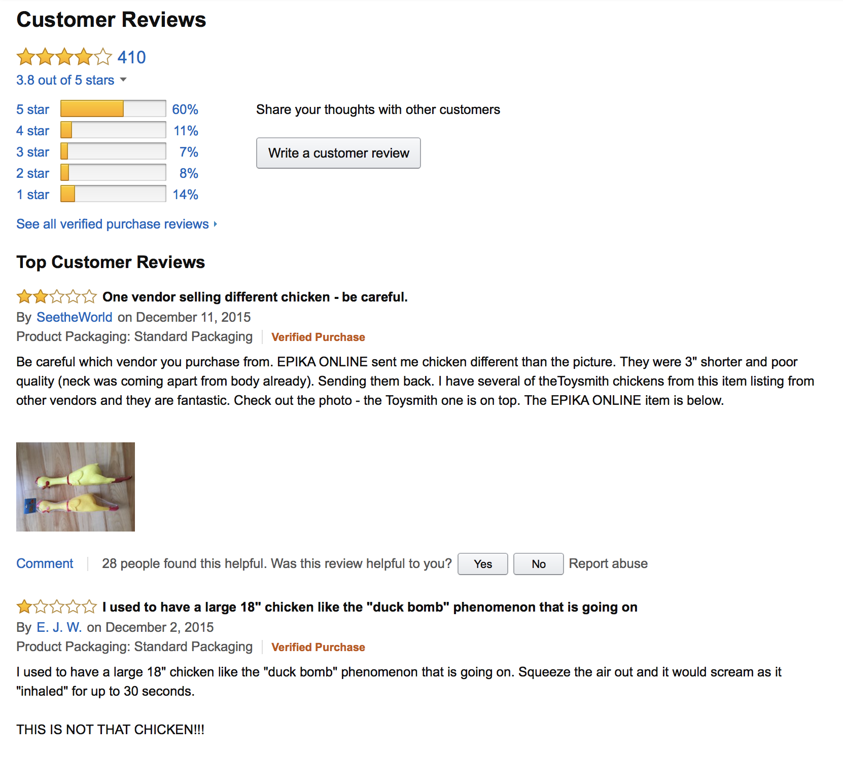
In the following, we will ask you to build statistical models to compare these two products using the observed rating. Larger versions of the images are available in the data set accompanying this notebook.

Exercise: Part I: A Maximum Likelihood Model

(Model Building) Suppose that for each product, we can model the probability of the value each new rating as the following vector:

\[ \theta = [\theta_1, \theta_2, \theta_3, \theta_4, \theta_5] \]

where $\theta_i$ is the probability that a given customer will give the product $i$ number of stars. That is, each new rating (a value between 1 and 5) has a categorical distribution $Cat(\theta)$. Represent the observed ratings of an Amazon product as a vector $R = [r_1, r_2, r_3, r_4, r_5]$ where, for example, $r_4$ is the number of $4$-star reviews out of a total of $N$ ratings. Write down the likelihood of $R$. That is, what is $p(R| \theta)$?

Note: The observed ratings for each product should be read off the image files included in the dataset.

Solution: Part I, Question 1

If each rating is distributed as a Categorical, then if we have $N$ number of independent observations of ratings and count up the total number $r_i$ for each star, then $R = [r_1, r_2, r_3, r_4, r_5]$ is distributed as a multinomial variable. That is, the likelihood for $R$ is

\[ \mathcal{L}(\theta) = \underbrace{\frac{n!}{r_1!\ldots r_5!} \theta_1^{r_1}\ldots \theta_5^{r_5}}_{\text{multinomial pdf}} \]

For Lotus, we estimate that the observed ratings vector is $[10\;\; 6\;\; 10\;\; 28\;\; 109]$ (depending on how you round, you might get a slightly different vector). Thus, the likelihood is

\[ \mathcal{L}_{\text{lotus}}(\theta) = \frac{n!}{10!6!10!28!109!} \theta_1^{10}\theta_2^{6}\theta_3^{10}\theta_4^{28}\theta_5^{109}. \]

For Toysmith, we estimate that the observed ratings vector is $[57\;\; 33\;\; 29\;\; 45\;\; 246]$. Thus, the likelihood is

\[ \mathcal{L}_{\text{toysmith}}(\theta) = \frac{n!}{57!33!29!45!246!} \theta_1^{57}\theta_2^{33}\theta_3^{29}\theta_4^{45}\theta_5^{246}. \]

(Model Fitting) Find the maximum likelihood estimator of $\theta$ for the Lotus World model; find the MLE of $\theta$ for the Toysmith model. You need to make a reasonably mathematical argument for why your estimate actually maximizes the likelihood (i.e. recall the criteria for a point to be a global optima of a function).

Note: I recommend deriving the MLE using the general expression of the likelihood. That is, derive the posterior using the variable $R$, then afterwards plug in your specific values of $R$ for each product.

Solution: Part I, Question 2

Recall that the MLE is defined as:

\[ \theta_{\text{MLE}} = \mathrm{argmax}_{\theta}\; \mathcal{L}(\theta). \]

Equivalently, the MLE can also be defined as:

\[ \theta_{\text{MLE}} = \mathrm{argmax}_{\theta}\; \log\mathcal{L}(\theta). \]

We will choose to work with the second definition since it involves a simpler objective function:

\[ \log\mathcal{L}(\theta) = \log[const] + \sum_{i=1}^5r_i\log\theta_i. \]

We need to remember that while we want to maximize the log-likelihood over $\theta$, we also need to ensure that $\theta$ defines a proper probability distribution over 5 categories, that is, $\sum_{i=1}^5 \theta_i = 1$. Thus, we must solve a constrained optimization problem:

\[ \max_{\theta}\; \log\mathcal{L}(\theta),\; \text{subject to }\sum_{i=1}^5 \theta_i = 1. \]

From Chapter 2, we know that the solution to the above problem must be a stationary point of the gradient of its corresponding Lagrangian:

\[ J(\theta, \lambda) = \log\mathcal{L}(\theta) - \lambda \left(\sum_{i=1}^5 \theta_i - 1\right). \]

Recall that the gradient of the Lagrangian is a vector of its partial derivatives:

\[ \nabla J = \left[\frac{\partial J}{\partial \theta_1} \ldots \frac{\partial J}{\partial \theta_5} \frac{\partial J}{\partial \lambda}\right] \]

Setting $\nabla J$ to zero and solving for $\theta, \lambda$ yield the stationary points:

\[\begin{split}\begin{aligned} \begin{cases} \frac{\partial J}{\partial \theta_i} = \frac{r_i}{\theta_i} - \lambda = 0&\\ \frac{\partial J}{\partial \lambda} = \sum_{i=1}^5 \theta_i - 1 = 0 \end{cases} \end{aligned}\end{split}\]

From the above, we see that the partial derivatives with respect to $\theta_i$ have a unique root at:

\[ \theta_i = \frac{r_i}{\lambda}, \]

substituting these solution into the equation $\sum_{i=1}^5 \theta_i - 1 = 0$ and solving for $\lambda$ yields

\[ \sum_{i=1}^5 r_i = \lambda. \]

Thus, the gradient of the Lagrangian has a unique stationary point at $\theta = [\theta_1 \ldots \theta_5]$, where

\[ \theta_i = \frac{r_i}{\sum_{i=1}^5 r_i}. \]

Since the log-likelihood is concave and the constraint is affine, at the unique stationary point we have the solution to the constrained optimization problem

\[ \max_{\theta}\; \log\mathcal{L}(\theta),\; \text{subject to }\sum_{i=1}^5 \theta_i = 1. \]

Therefore, the MLE of $\theta$ is given by

\[ \theta_{\text{MLE}} = \left[\frac{r_1}{\sum_{i=1}^5 r_i} \ldots \frac{r_5}{\sum_{i=1}^5 r_i}\right]. \]

Now we can use the observed ratings vector $R$ to compute the MLE of $\theta$ for each product.

\[\begin{split}\begin{aligned} \theta^{\text{lotus}}_{\text{MLE}} &= \left[\frac{10}{163}\; \frac{6}{163}\; \frac{10}{163}\; \frac{28}{163}\; \frac{109}{163}\right] = [.06\; .04\; .06\; .17\; .67]\\ \theta^{\text{toysmith}}_{\text{MLE}} &= \left[\frac{57}{410}\; \frac{33}{410}\; \frac{29}{410}\; \frac{45}{410}\; \frac{246}{410}\right] = [.14\; .08\; .07\; .11\; .6]\\ \end{aligned}\end{split}\]

Notice that these estimates of $\theta$ are precisely the percentages reported by Amazon to summarize the customer ratings! So this gives a reason for why reporting these percentage summaries are reasonable.

(Model Interpretation) Based on your MLE of $\theta$’s for both models, do you feel confident deciding if one product is superior to another? Why or why not?

Solution: Part I, Question 3

It is tempting to say that Lotus makes a better product since it receives, comparatively, a larger percentage of 4 and 5 star reviews; Lotus also receives, comparatively, a smaller percentage of 1 star reviews. But Lotus also has less than half the total number of reviews of Toysmith. It would be equally reasonable to argue that the lack of 1 star reviews, or some of the 4 or 5 star reviews for Lotus are “outliers”.

Exercise: Part II: A Bayesian Model

(Model Building) Suppose you are told that customer opinions are very polarized in the retail world of rubber chickens, that is, most reviews will be 5 stars or 1 stars (with little middle ground). What would be an appropriate $\alpha$ for the Dirichlet prior on $\theta$? Recall that the Dirichlet pdf is given by:

\[ p_{\Theta}(\theta) = \frac{1}{B(\alpha)} \prod_{i=1}^k \theta_i^{\alpha_i - 1}, \quad B(\alpha) = \frac{\prod_{i=1}^k\Gamma(\alpha_i)}{\Gamma\left(\sum_{i=1}^k\alpha_i\right)}, \]

where $\theta_i \in (0, 1)$ and $\sum_{i=1}^k \theta_i = 1$, $\alpha_i > 0 $ for $i = 1, \ldots, k$.

Solution: Part II, Question 1

Recall that the hyperparameters of the Dirichlet prior control the concentration of probability mass toward the five number 1, 2, 3, 4, 5. That is, if the prior is $\alpha = [1\; 1\; 1\; 1\; 1]$ then the probability mass is equally distributed on points where $\sum_{i=1}^5 \theta_i = 1$ with out biasing it towards any number, that is, $\theta$’s sampled from this Dirichlet will likely have equal values for $\theta_i$. If the prior is $\alpha = [100\; 1\; 1\; 1\; 1]$, then the probability mass will be skewed towards having higher values of $\theta_1$.

A plausible prior that reflects a very polarized customer base might be $\alpha = [100\; 1\; 1\; 1\; 100]$.

(Inference) Analytically derive the posterior distribution (using the likelihoods you derived in Part I) for each product.

Note: I recommend deriving the posterior using the general expression of a Dirichlet pdf. That is, derive the posterior using the variable $\alpha$, then afterwards plug in your specific values of $\alpha$ when you need to.

Solution: Part II, Question 2

The posterior $p(\theta|R)$ is given by

\[ p(\theta|R) = \frac{p(R | \theta) p(\theta)}{p(R)} = \frac{\frac{n!}{\prod_{i=1}^5 r_i!} \prod_{i=1}^5\theta_i^{r_i}* \frac{1}{B(\alpha)} \prod_{i=1}^5 \theta_i^{\alpha_i - 1}}{p(R)} \]

We can simplify the posterior as

\[\begin{split}\begin{aligned} p(\theta|R) &= \frac{const* \prod_{i=1}^5\theta_i^{r_i} \prod_{i=1}^5 \theta_i^{\alpha_i - 1}}{p(R)}\\ &= \frac{const* \prod_{i=1}^5\theta_i^{r_i} \theta_i^{\alpha_i - 1}}{p(R)}\\ &= \frac{const* \prod_{i=1}^5\theta_i^{\alpha_i + r_i - 1}}{p(R)}\\ &= const * \prod_{i=1}^5\theta_i^{\alpha_i + r_i - 1} \end{aligned}\end{split}\]

The posterior looks like another Dirichlet distribution $Dir(\alpha)$ with $\alpha = [\alpha_1 + r_1\;\; \alpha_2 + r_2\;\; \alpha_3 + r_3\;\; \alpha_4 + r_4\;\; \alpha_5 + r_5]$!

So, the posterior for Lotus is a Dirichlet with

\[ \alpha = [100 + 10\;\; 1 + 6 \;\; 1 + 10\;\; 1 + 28\;\; 100 + 109] = [110\;\; 7\;\; 11\;\; 29\;\; 209]; \]

the posterior for Toysmith is a Dirichlet with

\[ \alpha = [100 + 57\;\; 1 + 33\;\; 1 + 29\;\; 1 + 45\;\; 100 + 246] = [157\;\; 34\;\; 30\;\; 46\;\; 346]. \]

(The Maximum A Posterior Estimate) Analytically or empirically compute the MAP estimate of $\theta$ for each product, using the $\alpha$’s you chose in Question 1. How do these estimates compare with the MLE? Just for this problem, compute the MAP estimate of $\theta$ for each product using a Dirichlet prior with hyperparameters $\alpha = [1, 1, 1, 1, 1]$. Make a conjecture about the effect of the prior on the difference between the MAP estimates and the MLE’s of $\theta$.

Solution: Part II, Question 3

The MAP estimate is the mode of the posterior. Since the posteriors are Dirichlet, the modes are given by:

\[ \theta_i = \frac{\alpha_i - 1}{\sum_{i=1}^5 \alpha_i - 5}, \text{ if $\alpha_i > 1$} \]

Thus, we can compute

\[\begin{split}\begin{aligned} \theta^{\text{lotus}}_{\text{MAP}} &= [0.3\;\;0.017\;\;0.028\;\;0.078\;\;0.58]\\ \theta^{\text{toysmith}}_{\text{MAP}} &= [0.26\;\;0.054\;\;0.048\;\;0.074\;\;0.57] \end{aligned}\end{split}\]

Recall that the MLE of the $\theta$’s are

\[\begin{split}\begin{aligned} \theta^{\text{lotus}}_{\text{MLE}} &= [0.06\; 0.04\; 0.06\; 0.17\; 0.67]\\ \theta^{\text{toysmith}}_{\text{MLE}} &= [0.14\; 0.08\; 0.07\; 0.11\; 0.6]\\ \end{aligned}\end{split}\]

We see that $\theta^{\text{lotus}}_{\text{MAP}}$ lowered the probability for 5-star ratings and increased the probability of 1-star ratings, by a large margin. While $\theta^{\text{toysmith}}_{\text{MAP}}$ lowered the probability for 5-star ratings and increased the probability of 1-star ratings by a smaller amount. For both products, the MAP estimate lowered the probability of non-extreme ratings (2-4 stars). This trend makes sense since our prior assumes that customers tend to give extreme ratings. Under the MAP estimates of $\theta$, we see that Lotus has less of an obvious advantage – the probability of 5-star ratings for both products are now similar.

Rather than analytically computing the posterior mode, we can find it empirically. That is, we can sample from the posterior and compute the most likely value for these samples. Typically this is done by binning the samples along the domain space and selecting the bin with the largest number of samples. There are a number of numpy and scipy functions that will perform the binning. The accuracy of your estimate of the mode depends on the granularity of the bins (for example, if you’re building a 1-D histogram with two bins your mode estimate will be way off, where as a histogram with 100 bins might perform better). In this case, for simplicity, we estimate the posterior mode by sampling from the posterior and histogramming each component $\theta_i$ of the samples. In general, the mode of a joint distribution cannot be estimated by taking the mode of the individual marginals. However, since the Dirichlet distribution is unimodal when $\alpha_i> 1$, this estimation, while crude, is not unreasonable.

samples = 5000
#sample from the lotus posterior
lotus_posterior_samples = np.random.dirichlet([110, 7, 11, 29, 209], size=samples)
#sample from the toysmith posterior
toysmith_posterior_samples = np.random.dirichlet([157, 34, 30, 46, 346], size=samples)

#visualize these posterior samples
fig, ax = plt.subplots(2, 5, figsize=(25, 10))
for i in range(5):
    ax[0, i].hist(lotus_posterior_samples[:, i], bins=50, color='blue', alpha=0.6)
    ax[0, i].set_title('Lotus: histogram of posterior samples of theta_{}'.format(i))
for i in range(5):
    ax[1, i].hist(toysmith_posterior_samples[:, i], bins=50, color='red', alpha=0.6)
    ax[1, i].set_title('Toysmith: histogram of posterior samples of theta_{}'.format(i))
plt.tight_layout()
plt.show()

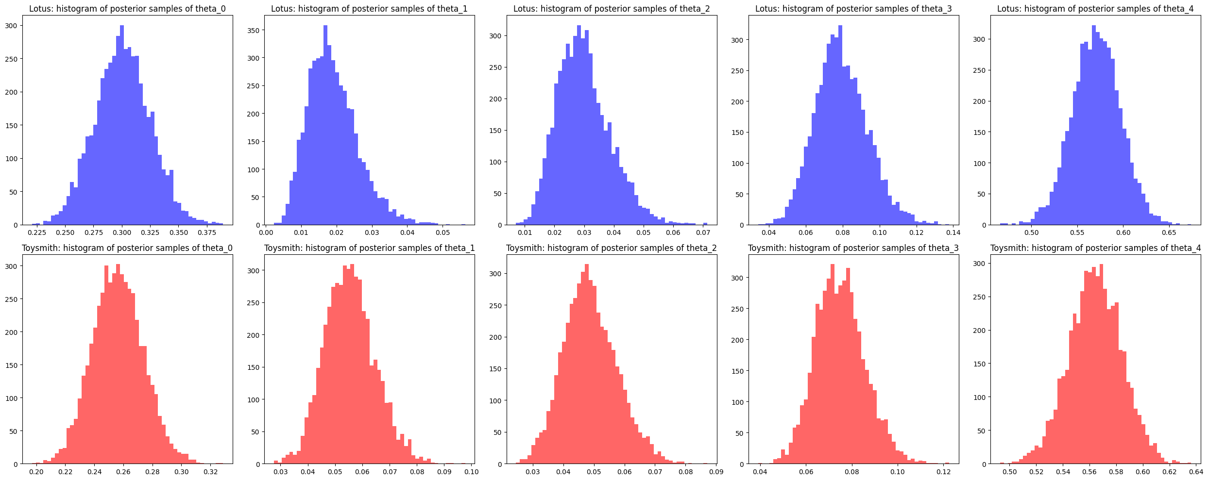
We see that the mode of the posterior samples closely resemble the MAP estimates we derived analytically for each product.

Not covered here: the MAP estimates under the uniform prior $\alpha = [1, 1, 1, 1, 1]$, and the conjecture about the effect of the prior.

(The Posterior Mean Estimate) Analytically or empirically compute the posterior mean estimate of $\theta$ for each product, using the $\alpha$’s you chose in Question 1. How do these estimates compare with the MAP estimates and the MLE?

Solution: Part II, Question 4

The means of our Dirichlet distribution is given by

\[ \frac{\alpha_i}{\sum_{i=1}^5 \alpha_i}. \]

Thus, we can compute

\[\begin{split}\begin{aligned} \theta^{\text{lotus}}_{\text{Post Mean}} &= [0.3, 0.019, 0.03, 0.079, 0.57]\\ \theta^{\text{toysmith}}_{\text{Post Mean}} &= [0.26, 0.055, 0.049, 0.075, 0.56] \end{aligned}\end{split}\]

These estimates are very similar to the MAP estimates and are quite different from the MLE.

Again, we can empirically estimate the posterior mean. That is, we sample from the posterior and compute the mean of those samples.

lotus_posterior_mean = lotus_posterior_samples.mean(axis=0)
toysmith_posterior_mean = toysmith_posterior_samples.mean(axis=0)

print('lotus', lotus_posterior_mean)
print('toysmith', toysmith_posterior_mean)

lotus [0.30082613 0.01903371 0.02991358 0.07938425 0.57084233]
toysmith [0.2562429  0.05545415 0.04880784 0.07501581 0.5644793 ]

Again, we see that the empirical estimates of the posterior means are similar to the values we derived analytically.

(The Posterior Predictive Estimate) Sample 1000 rating vectors from the posterior predictive for each product, using the $\alpha$’s you chose in Question 1. Use the average of the posterior predictive samples to estimate $\theta$. How do these estimates compare with the MAP, MLE, posterior mean estimate of $\theta$?

Solution: Part II, Question 5

To sample from the posterior predictive, we sample $N$ samples of $\theta$ from the posterior. Each sample of $\theta$ parametrizes a distinct multinomial model. We sample an outcome $Y$ from each of these models. Taking the average value of these samples, we can estimate the percentage of 1-star reviews, 2-star reviews etc.

lotus_posterior_pred = np.array([np.random.multinomial(163, sample, size=1)[0] for sample in lotus_posterior_samples])
toysmith_posterior_pred = np.array([np.random.multinomial(410, sample, size=1)[0] for sample in toysmith_posterior_samples])

lotus_posterior_pred_mean = lotus_posterior_pred.mean(axis=0)
toysmith_posterior_pred_mean = toysmith_posterior_pred.mean(axis=0)

print('lotus', lotus_posterior_pred_mean)
print('toysmith', toysmith_posterior_pred_mean)

lotus [49.006   3.137   4.8936 12.8978 93.0656]
toysmith [104.917   22.8216  20.1068  30.6664 231.4882]

lotus_posterior_pred_mean_percent = lotus_posterior_pred_mean / lotus_posterior_pred_mean.sum()
toysmith_posterior_pred_mean_percent = toysmith_posterior_pred_mean / toysmith_posterior_pred_mean.sum()

print('lotus', lotus_posterior_pred_mean_percent)
print('toysmith', toysmith_posterior_pred_mean_percent)

lotus [0.30065031 0.0192454  0.03002209 0.07912761 0.5709546 ]
toysmith [0.25589512 0.05566244 0.04904098 0.0747961  0.56460537]

It looks like that the percentages of star ratings estimated from the posterior predictive are very similar to the MAP and posterior mean estimates of the $\theta$’s of the two products!

(Model Evaluation) Compute the 95% credible interval of $\theta$ for each product (Hint: compute the 95% credible interval for each $\theta_i$, $i=1, \ldots, 5$). For which product is the posterior mean and MAP estimate more reliable and why?

Solution: Part II, Question 6

Just as in the Chapter 1 problem set, we empirically compute the 95% credible interval for $\theta$ by sampling from the posterior and then taking the empirical 95% interval of the samples. Again, we estimate the interval for $\theta$ by estimating the 95% credible interval of each $\theta_i$ from the posterior marginal distribution.

Note that this is again a simplification. The multivariate version of $n\%$ credible intervals is credible region, a region in the parameter space over which contains n% of the pdf’s probability mass. A 95% confidence region for a general joint posterior distribution may not be a box but, rather, a complex shape. Our approximation of the 95% confidence region by the confidence intervals of the marginal posterior distributions defines a bounding box around this region and, in general, may be wider than necessary.

lotus_lb = np.percentile(lotus_posterior_samples, 2.5, axis=0)
lotus_ub= np.percentile(lotus_posterior_samples, 97.5, axis=0)

toysmith_lb = np.percentile(toysmith_posterior_samples, 2.5, axis=0)
toysmiths_ub = np.percentile(toysmith_posterior_samples, 97.5, axis=0)

print('lotus 2.5%', lotus_lb)
print('lotus 97.5%', lotus_ub)
print('\n')
print('toysmith 2.5%', toysmith_lb)
print('toysmith 97.5%', toysmiths_ub)

lotus 2.5% [0.25415424 0.00760864 0.01505252 0.05351941 0.51903437]
lotus 97.5% [0.34898777 0.03499885 0.04965096 0.10971106 0.62179894]


toysmith 2.5% [0.22292189 0.03885184 0.03290497 0.05534909 0.52540982]
toysmith 97.5% [0.29125427 0.07495462 0.06735598 0.09737386 0.60327188]

We see that the credible intervals for both products have comparable width – i.e. no model is more “certain” about $\theta$ than the other.

Since the confidence intervals (especially for the 5-star probability and the 1-star probability) overlap a great deal it may be unreasonable to use our point estimates (MAP, MLE etc) to rank the two products.

Exercise: Part III: Broader Impact Analysis

Starting in 2020, major machine learning conferences are beginning to ask authors as well as reviewers to explicitly consider the broader impact of new machine learning methods. To properly evaluate the potential good or harm that a piece of technology (AI or not) can do to the general public, we need to be aware that no technology is deployed in ideal conditions or in perfectly neutral contexts. In order to assess the potential broader impact of technology, we need to analyze the social systems/institutions of which these technologies will become a part.

To help you analyze the broader impact of your technology, begin by considering the following questions:

I. Identify the relevant socio-technical systems

In what social, political, economic system could the tech be deployed?
How would the tech be used in these systems (what role will it take in the decision making processes)?

II. Identify the stakeholders

Who are the users?
Who are the affected communities (are these the users)?

Hint: users are typically decision makers who will use the technology as decision aids (e.g. doctors), whereas affected communities may be folks who are impacted by these decisions but who are not represented in the decision making process (e.g. patients).

III. What types of harm can this tech do?

What kinds of failures can this tech have?
What kinds of direct harm can these failures cause?
What kinds of harm can the socio-technical system cause?

Hint: many technical innovations have niche applications, they may sit in a long chain of decision making in a complex system. As such, it may seem, at first glance, that these technologies have no immediate real-life impact. In these cases, it’s helpful to think about the impact of the entire system and then think about how the proposed innovations aid, hamper or change the goals or outcomes of this system.

IV. What types of good can this tech do?

What kinds of needs do these users/communities have?
What kinds of constraints do these users/communities have?

(Impact) Analyze the broader impact of models of product popularity/quality when used for ranking. Specifically, focus on anticipating ways these models can interact with other components of the decision systems in which they will be deployed, identifying end-users, affected communities as well as anticipating the effects (positive and negative) on affected communities (in particular, does the model have the same effect on all subpopulations in the affected communities?).

(Comparison of Ranking Systems)

Recall that on Amazon, the first customer review statistic displayed for a product is the average rating. What is potentially problematic with ranking products based on the average customer rating?

Which point estimate (MAP, MLE, posterior mean or posterior predictive estimate) of $\theta$, if any, would you feel choose to rank the two Amazon products? Why?

Hint: think about which of these estimates are equivalent (if any). If they are not equivalent, what are the special properties of each estimate? What aspect of the data or the model is each estimate good at capturing?

Note: we’re not looking for “the correct answer” here. We are looking for a sound decision based on a statistically correct interpretation of your models.

Solution: Part III, Question 2

There are two immediate issues with using an “average star rating” to rank products:

An average star rating can obscure the difference between a mediocre product (one that receives 100 two or three star reviews) and a polarizing product (one that receives 50 five star reviews and 50 one star reviews). We can, no doubt, all think of instances where distinguishing between a mediocre product and a polarizing product makes all the difference in the world (to consumers).
Another problem with averaging star ratings is a general statistical weakness of using averages to rate things. We’ve seen this problem pop up in many previous examples, when small sample sizes heavily skew averages towards extreme values.

Not covered here: which point estimate of $\theta$, if any, to use to rank the two products.

3.7. Further Reading#

Statistics

(Introductory) Philosophy and the practice of Bayesian statistics
(Introductory) The Exponential Family: Conjugate Priors

Other Reference

Gelman, Chapters 2 & 3
Gelman, Chapter 4

Bayesian Modeling

Contents

3. Bayesian Modeling#

3.1. Review of the Method of Maximum Likelihood#

The Method of Maximum Likelihood#

Evaluating the MLE#

Properties of The Maximum Likelihood Estimator#

Is Bias Always Bad?#

Limitations of MLE: Overfitting Under Scarcity of Data#

Regularization#

3.2. Models for Real Data#

Video Ranking#

Kidney Cancer Rates#

Birth Weights#

3.3. The Beta-Binomial Model#

The Coin Toss Model: Revisited#

Incorporating Prior Beliefs#

The Beta-Binomial Model#

Posterior for the Beta-Binomial Model#

Interpreting the Posterior: Bayesian Update#

Simulation: Bayesian Update for the Coin Flip#

Making Predictions#

Simulation: Posterior Predictive for the Coin Flip#

3.4. Bayesian Modeling - A Summary#

The Bayesian Modeling Process#

Evaluating Bayesian Models#

Where do Priors Come From?#

3.5. Summary#

3.6. Exercises#

Problem Set: Review of Statistical Modeling and Scientific Computing#

Problem Description#

3.7. Further Reading#