13. Hierarchical Models

This chapter is adapted from AM207 (Harvard, Fall 2021). Watch the recorded lecture.

Show code cell content

Hide code cell content

#--------  movie_stats
# A function that extracts the number of likes and total number of ratings for a movie
# Input: 
#      movie_name (an optional parameter containing the exact name of the movie)
#      movie_name_contains (an optional parameter containing a portion of the name of the movie)
# Returns: 
#      total_ratings (the total number of ratings for a movie)
#      likes (the total number of likes for a movie)

def movie_stats(movie_name=None, movie_name_contains=None):
    
    #If given an exact movie name:
    if movie_name is not None:        
        #Find the index of the movie, by name, in the "names" dataframe
        movie_index = names_df[names_df['movie_name'] == movie_name].index[0]
        #Get the id for the movie in the "names" dataframe
        movie_id = names_df.loc[movie_index, 'movie_id']
        #Get all ratings for the movie, by id, in the "ratings" dataframe
        ratings_for_movie = ratings_df[ratings_df['movie_id'] == movie_id]
        #Count the total number of ratings
        total_ratings = len(ratings_for_movie)
        #Count the likes (the 1's)
        likes = ratings_for_movie['rating'].sum()
    
    #Otherwise, if given a partial movie name:
    elif movie_name_contains is not None:
        #Find the index of the movie, by name, in the "names" dataframe
        movie_index = names_df[names_df['movie_name'].str.contains(movie_name_contains)].index[0]
        #Get the id for the movie in the "names" dataframe
        movie_id = names_df.loc[movie_index, 'movie_id']
        #Get all ratings for the movie, by id, in the "ratings" dataframe
        ratings_for_movie = ratings_df[ratings_df['movie_id'] == movie_id]
        #Count the total number of ratings
        total_ratings = len(ratings_for_movie)
        #Count the likes (the 1's)
        likes = ratings_for_movie['rating'].sum()
    
    else:
        total_ratings = 0.
        likes = 0.
    
    return float(total_ratings), likes

#--------  plot_beta_prior
# A function to visualize a beta pdf on a set of axes
# Input: 
#      a (parameter controlling shape of beta prior)
#      b (parameter controlling shape of beta prior)
#      color (color of beta pdf)
#      ax (axes on which to plot pdf)
# Returns: 
#      ax (axes with plot of beta pdf)

def plot_beta_prior(a, b, color, ax):
    
    #Create a beta-distributed random variable with shape a, b
    rv = sp.stats.beta(a, b)
    #Create values from 0 to 1
    x = np.linspace(0, 1, 100)
    #Plot the beta pdf for values from 0 to 1
    ax.plot(x, rv.pdf(x), '-', lw=2, color=color, label='a=' + str(a) + ', b=' + str(b))
    #Set title, legend etc
    ax.set_title('Beta prior with a=' + str(a) + ', b=' + str(b))
    ax.legend(loc='best')
    
    return ax

#--------  sample_posterior
# A function that samples points from the posterior over a movie's 
# likability, given a binomial likelihood function and beta prior
# Input: 
#      a (parameter controlling shape of beta prior)
#      b (parameter controlling shape of beta prior)
#      likes (the number of likes in likelihood)
#      ratings (total number of ratings in likelihood)
#      n_samples (number of samples to take from posterior)
# Returns: 
#      post_samples (a array of points from the posterior)

def sample_posterior(a, b, likes, ratings, n_samples):
    #Samples points from a beta distribution 
    #(the posterior of a binomial likelihood and a beta prior is a beta distribution!)
    post_samples = np.random.beta(a + likes, b + ratings - likes, n_samples)
    return post_samples


#--------  find_mode
# A function that approximates the mode of a distribution given a sample from the distribution
# Input: 
#      values (samples from the distribution)
#      num_bins (number of bins to use in approximating histogram)
# Returns: 
#      mode (the approximate mode of the distribution)

def find_mode(values, num_bins):
    
    #Make an approximation (histogram) of the distribution using the samples
    bins, edges = np.histogram(values, bins=num_bins)
    #Find the bin in the histogram with the max height
    max_height_index = np.argmax(bins)
    #Find the sample corresponding to the bin with the max height (the mode)
    mode = (edges[max_height_index] + edges[max_height_index + 1]) / 2.
    
    return mode


def plot_priors_with_posteriors(ax, beta_shapes, likes, total_ratings, n_samples):
    #Start the index of the current subplot at 0
    ax_ind = 0
    #Iterate through all the shapes
    for a, b in beta_shapes:
        #Plot the beta pdf for a particular shape
        plot_beta_prior(a, b, 'blue', ax[0, ax_ind])
        #Increment the subplot index
          
        #Draw samples from the posterior corresponding to a particular beta prior
        post_samples = sample_posterior(a, b, likes, total_ratings, n_samples)
        #Approximate the posterior with a histogram of these samples
        ax[1, ax_ind].hist(post_samples, bins=30, color='red', alpha=0.5)
        #Find the approximate mode of the posterior
        mode = find_mode(post_samples, 30)
        #Plot the mode as a vertical line
        ax[1, ax_ind].axvline(x=mode, linewidth=3, label='Posterior mode')

        #Set title, legends etc
        ax[1, ax_ind].set_title('Posterior, with Beta prior (a={}, b={})'.format(a, b))
        ax[1, ax_ind].legend(loc='best')
        #Increment the subplot index
        ax_ind += 1
        
    return ax

In this chapter

1. Review of Statistical Modeling

2. Motivation for Hierarchical Models

3. Hierarchical Models and Empirical Bayes

Show code cell content

Hide code cell content

### Import basic libraries
import numpy as np
import scipy as sp
from scipy.special import logsumexp
import pandas as pd
import sklearn as sk
from sklearn.linear_model import LinearRegression
from sklearn.preprocessing import PolynomialFeatures
import matplotlib.pyplot as plt
%matplotlib inline

13.1. Review of Statistical Modeling

What We Can Do So Far: Models

1. (Likelihood Models with Observed Variables) When we have observed data \(Y_{\text{Obs}}\), we can model \(Y_{\text{Obs}}\) as a random variable \(Y_{\text{Obs}} \sim p(Y |\theta)\) with a known distribution \(p\).

   • if \(Y_{\text{Obs}}\) is a label, we can model it as a Categorical or Bernoulli variable

   • if \(Y_{\text{Obs}}\) is a count, we can model it as a Binomial, Multinomial or Poisson

   • if \(Y_{\text{Obs}}\) is continuous, we can model it as a Gaussian, Exponential, Dirichlet etc
     
     

2. (Likelihood Models with Latent Variables) When we also have unobserved data \(Z_{\text{Latent}}\), we can model \(Z_{\text{Latent}}\) and \(Y_{\text{Obs}}\) jointly \(p(Y_{\text{Obs}}, Z_{\text{Latent}}| \theta)\).
   
   

3. (Bayesian Models) When we are being Bayesian, we assume a prior for \(\theta\), encoding our knowledge and uncertainty about \(\theta\). We model parameters and data jointly \(p(Y_{\text{Obs}}, \theta)\) or \(p(Y_{\text{Obs}}, Z_{\text{Latent}}, \theta)\).

What We Can Do So Far: Inference

We can make statements about \(\theta\) by performing:

I. Maximum Likelihood Estimation: for likelihood models, we compute a fixed value \(\theta_{\text{MLE}}\) that maximizes the likelihood of the observed data \(Y\).

II. Bayesian Inference: for Bayesian models, we compute the posterior distribution \(p(\theta| Y)\).

We choose an inference algorithm or method to perform inference:

I. Maximum Likelihood Estimation:
A. For models with observed variables, we analytically solve an unconstrained or constrained optimization problem to obtain \(\theta_{\text{MLE}}\).
B. For latent variable models, we use expectation maximization to approximately find \(\theta_{\text{MLE}}\).

II. Bayesian Inference:
A. If the prior and likelihood are conjugate, analytically derive the posterior distribution
B. If the posterior distribution does not have a known form, sample from it using a sampler.
C. If the posterior distribution does not have a known form, approximate it using variational inference.

What Can We Not Do?

1. (Regression Models) We don’t have any models where some observed variables \(Y_{\text{Obs}}\) depend on other observed variables \(X_{\text{Obs}}\), i.e. none of our models have covariates that we condition on.

2. (Gradient Descent Methods) Analytically optimizing the log-likelihood is not always possible, and when possible it is extremely annoying to do by hand. Can we find a way to black-box optimize any objective function?

3. (Hamiltonian Monte Carlo) MCMC samplers can be extremely inefficient in high-dimensions where the samplers struggle to find area of high mass in the target distribution. Can we build a proposal distribution with an indicator of where the target distribution mass is located?

4. (Black-box Variational Inference etc) Variational inference sounds like a great idea but maximizing the ELBO using coordinate ascent is an artisanal process that requires a massive amount of derivations per model. Can we find an algorithm to compute/estimate the gradient of the ELBO that is model independent? Can we perform black-box variational inference?

What Happens After Inference?

1. (Predictive Evaluation) In practice, we do not know the true model \(\theta_{\text{True}}\)! Thus, \(\theta_{\text{MLE}}\) and \(p(\theta|Y)\) cannot be evaluated by comparison to \(\theta_{\text{True}}\).

   • Maximum Likelihood Estimation: we compute \(\theta_{\text{MLE}}\) on multiple bootstrap samples of the data; for each \(\theta_{\text{MLE}}\) we sample \(Y \sim p(Y| \theta_{\text{MLE}})\). We compare these samples with observed data \(Y_{\text{Obs}}\).

   • Bayesian Inference: we sample \(\theta\)’s from the posterior, for each \(\theta\sim p(\theta |Y_{\text{Obs}})\) we sample \(Y \sim p(Y| \theta)\). We compare these posterior predictive samples with the observed data \(Y_{\text{Obs}}\).
     
     

2. (Uncertainty Evaluation) Before making decisions with real-life consequence based on your model, you should check the precision of your estimate or uncertainty of you model.

   • Maximum Likelihood Estimation: repeat the MLE computation on many bootstrap samples of \(Y_{\text{Obs}}\). Compute the confidence interval of \(\theta\) and the predictive interval for \(Y\). These intervals indicate precision.

   • Bayesian Inference: Compute credible intervals for the posterior \(p(\theta|Y)\) and the predictive intervals of the posterior predictive. These intervals indicate model uncertainty.

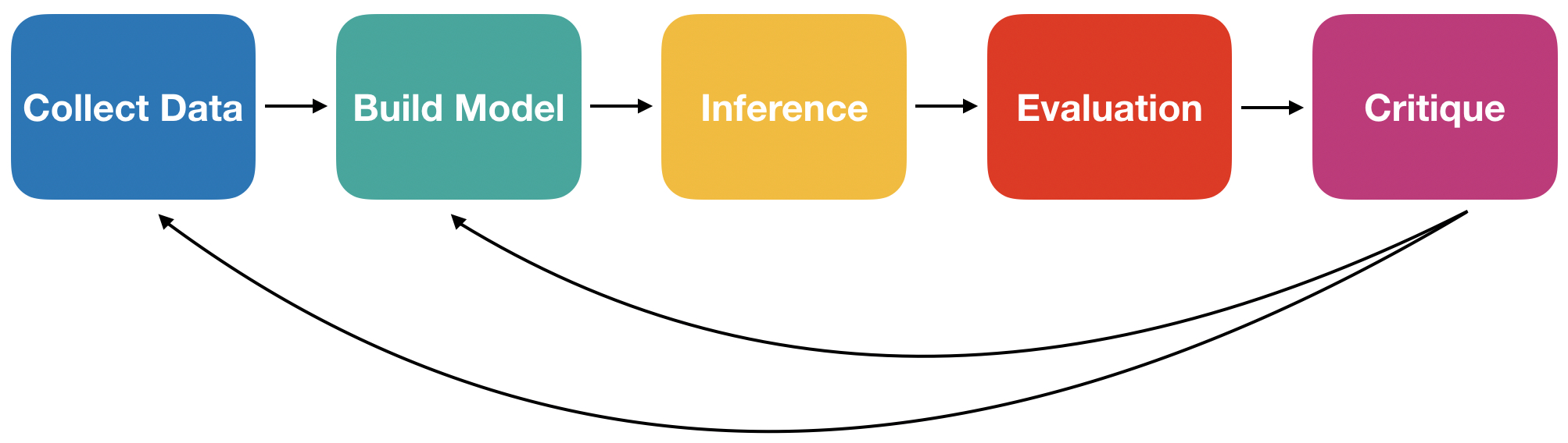
The Modeling Process

Evaluating the Predictive Distributions

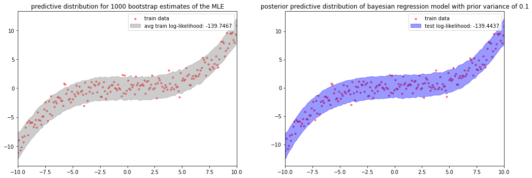
How well does the predictive distribution of bootstrapped MLE models or the posterior predictive of a Bayesian model capture the actual observed data?

We cannot, in general, perform visual checks (i.e. plot the predictive and the data). To quantify how well a predictive distribution aligns with the actual data we can compute:

1. The KL-divergence between actual data (empirical distribution) and our predictive distribution.

2. The log-likelihood of the actual data.

   A. For MLE models: we can compute \(\log p(Y^{\text{Obs}}| \theta_{\text{MLE}})\) for each bootstrap \(\theta_{\text{MLE}}\) and then average the log-likelihood over the number of bootstraps. If there are multiple observations, we would sum the individual log-likelihoods at the end.
   
   

   B. For Bayesian models: we evaluate the log-likelihood, i.e the likelihood of the observed data under the posterior predictive,

   \[ \log \prod_{n=1}^N \int_{\Theta} p(Y^{\text{Obs}}_n | \theta) p(\theta|Y^{\text{Obs}}_1, \ldots, Y^{\text{Obs}}_N) d\theta \approx \sum_{n=1}^N\log \frac{1}{S} \sum_{s=1}^S p(Y^{\text{Obs}}_n | \theta_s), \]

   where \(\theta_s\sim p(\theta|Y^{\text{Obs}}_1, \ldots, Y^{\text{Obs}}_N)\)

Show code cell content

Hide code cell content

## generate training data
#number of points in each of the two segments of the domain
N = 100
#training x
x_1 = np.hstack((np.linspace(-10, -5, N), np.linspace(5, 10, N)))
x_2 = np.linspace(-10, 10, 2 * N)
#output noise variance
y_var = 1.0
#function relating x and y
f = lambda x:  0.01 * x**3
#y is equal to f(x) plus gaussian noise
y_1 = f(x_1) + np.random.normal(0, y_var, 2 * N)
y_2 = f(x_2) + np.random.normal(0, y_var, 2 * N)

#prior variance for the bayesian model
prior_var = 0.5

## generate testing data
#nubmer of testing points
N_test = 100
#testing x
x_test = np.linspace(-10, 10, N_test)
y_test = f(x_test) + np.random.normal(0, y_var, N_test)

#total number of bootstrap estimates of the MLE
trials = 1000
#set up for polynomial (deg 7) regression
linear_model = LinearRegression()
poly = PolynomialFeatures(7)

Show code cell content

Hide code cell content

def mle_vs_bayesian(x, y, ax, prior_var=1.):
    #transform training x: add polynomial features
    x_poly = poly.fit_transform(x.reshape((-1, 1)))
    #transform x_test: add polynomial features
    x_test_poly = poly.fit_transform(x_test.reshape((-1, 1)))
    #Gaussian log pdf
    gaussian_log_pdf = lambda mu, sigma_sq, x: -0.5 * (np.log(2 * np.pi * sigma_sq) + (x - mu)**2 / sigma_sq)
    
    ##fit mle on multiple bootstraps
    log_likelihood = []
    y_predict = []
    for n in range(trials):
        #create bootstrap sample from data
        x_bootstrap = np.random.choice(x, size=len(x), replace=True)
        #add polynomial features
        x_bootstrap_poly = poly.fit_transform(x_bootstrap.reshape((-1, 1)))
        #compute MLE for the coefficients/parameters of the polynomial model 
        linear_model.fit(x_bootstrap_poly, f(x_bootstrap) + np.random.normal(0, y_var, 2 * N))
        #predict on x_test using your MLE model
        prediction = linear_model.predict(x_test_poly)
        y_predict.append(prediction + np.random.normal(0, y_var, N_test))
        #compute log-likelihood of test data
        log_likelihood.append(gaussian_log_pdf(prediction, y_var, y_test).sum())
    y_predict = np.array(y_predict)
    log_likelihood = np.array(log_likelihood).mean()
    
    #compute the 95 percentiles of the predictions
    ub = np.percentile(y_predict, 97.5, axis=0)
    lb = np.percentile(y_predict, 2.5, axis=0)
    
    ax[0].scatter(x, y, color='red', s=10, alpha=0.5, label='train data')
    #ax[0].scatter(x_test, y_test, color='black', s=10, alpha=0.5, label='test data')
    ax[0].fill_between(x_test, ub, lb, color='gray', alpha=0.4, label="avg train log-likelihood: {}".format(np.round(log_likelihood, 4)))
    ax[0].set_title('predictive distribution for {} bootstrap estimates of the MLE'.format(trials))
    ax[0].legend(loc='best')
    ax[0].set_xlim([-10, 10])
    
    #number of samples from the posterior
    S = trials
    #add a column of one's representing the bias
    x_matrix = np.hstack((x_poly, np.ones((x_poly.shape[0], 1))))
    #add a column of one's representing the bias
    x_test_matrix = np.hstack((x_test_poly, np.ones((x_test_poly.shape[0], 1))))
    #reshape y into 2D array
    y_matrix = y.reshape((-1, 1))

    prior_variance = np.diag(prior_var * np.ones(x_matrix.shape[1]))
    prior_precision = np.linalg.inv(prior_variance)

    joint_precision = prior_precision + x_matrix.T.dot(x_matrix) / y_var
    joint_variance = np.linalg.inv(joint_precision)
    joint_mean = joint_variance.dot(x_matrix.T.dot(y_matrix)) / y_var

    #sampling S points from the posterior
    posterior_samples = np.random.multivariate_normal(joint_mean.flatten(), joint_variance, size=S)
    #sampling S points from the posterior predictive
    y_predict_noiseless = np.array([x_test_matrix.dot(sample) for sample in posterior_samples])
    y_predict_bayes = y_predict_noiseless + np.random.normal(0, y_var, size=(S, N_test))
    
    log_likelihood_bayes = []
    #compute log likelihood for the test data
    for n in range(len(y_test)):
        log_likelihood_bayes.append(logsumexp(gaussian_log_pdf(y_test[n], y_var, y_predict_noiseless[:, n])))
    log_likelihood_bayes = np.array(log_likelihood_bayes).sum() - len(y_test) * np.log(S)

    #compute the 95 percentiles of the posterior predictives
    ub_bayes = np.percentile(y_predict_bayes, 97.5, axis=0)
    lb_bayes = np.percentile(y_predict_bayes, 2.5, axis=0)
    
    ax[1].scatter(x, y, color='red', s=10, alpha=0.5, label='train data')
    #ax[1].scatter(x_test, y_test, color='black', s=10, alpha=0.5, label='test data')
    ax[1].fill_between(x_test, ub_bayes, lb_bayes, color='blue', alpha=0.4, label="test log-likelihood: {}".format(np.round(log_likelihood_bayes, 4)))
    ax[1].set_title('posterior predictive distribution of bayesian regression model with prior variance of {}'.format(prior_var))
    ax[1].legend(loc='best')
    ax[1].set_xlim([-10, 10])
    
    return ax

Interpreting the Data Log-Likelihood

fig, ax = plt.subplots(1, 2, figsize=(15, 5))
prior_var = 0.1
ax = mle_vs_bayesian(x_2, y_2, ax, prior_var=prior_var)
plt.tight_layout()
plt.show()

Evaluating and Quantifying Uncertainty

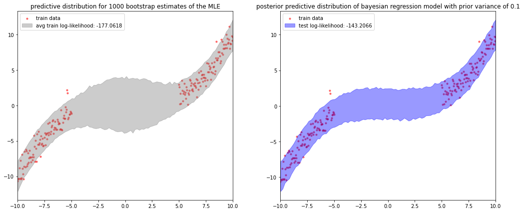
How do we know our model uncertainties (confidence intervals, credible intervals, predictive intervals, posterior predictive intervals) are any good? What information about the data/model do we want our uncertainties to capture?

Epistemic Uncertainty: uncertainty due to small number of samples across all scenarios. This can be reduced by more samples!

Aleatoric Uncertainty: uncertainty due to the underlying randomness of the data generation process. This cannot be reduced no matter what.

Can we use log-likelihood of as a metric for the quality of predictive uncertainty?

fig, ax = plt.subplots(1, 2, figsize=(15, 6))
ax = mle_vs_bayesian(x_1, y_1, ax, prior_var=prior_var)
plt.tight_layout()
plt.show()

13.2. Motivation for Hierarchical Models

A Binomial Model for Movie Rankings

We model the number of likes \(Y_n\) received by the \(n\)-th movie as a binomial variable \(Y_n | \theta_n\sim Bin(R_n, \theta_n)\), where \(R_n\) is the number of times the \(n\)-th movies was rated and \(\theta_n\) is the “likeability” of the movie.

Show code cell source

Hide code cell source

ratings_df = pd.read_csv('../data/dataset_4_ratings.txt', delimiter=',')
ratings_df.head()

	user_id	movie_id	rating
0	22.0	377.0	0.0
1	62.0	257.0	0.0
2	95.0	546.0	0.0
3	38.0	95.0	1.0
4	63.0	277.0	1.0

Show code cell source

Hide code cell source

names_df = pd.read_csv('../data/dataset_4_movie_names.txt', delimiter='|', encoding = "ISO-8859-1")
names_df.head()

	movie_id	movie_name	release_date	Unnamed: 3	link	Unnamed: 5	Unnamed: 6	Unnamed: 7	Unnamed: 8	Unnamed: 9	...	Unnamed: 15	Unnamed: 16	Unnamed: 17	Unnamed: 18	Unnamed: 19	Unnamed: 20	Unnamed: 21	Unnamed: 22	Unnamed: 23	Unnamed: 24
0	1	Toy Story (1995)	01-Jan-1995	NaN	http://us.imdb.com/M/title-exact?Toy%20Story%2...	0	0	0	1	1	...	0	0	0	0	0	0	0	0	0	NaN
1	2	GoldenEye (1995)	01-Jan-1995	NaN	http://us.imdb.com/M/title-exact?GoldenEye%20(...	0	1	1	0	0	...	0	0	0	0	0	0	1	0	0	NaN
2	3	Four Rooms (1995)	01-Jan-1995	NaN	http://us.imdb.com/M/title-exact?Four%20Rooms%...	0	0	0	0	0	...	0	0	0	0	0	0	1	0	0	NaN
3	4	Get Shorty (1995)	01-Jan-1995	NaN	http://us.imdb.com/M/title-exact?Get%20Shorty%...	0	1	0	0	0	...	0	0	0	0	0	0	0	0	0	NaN
4	5	Copycat (1995)	01-Jan-1995	NaN	http://us.imdb.com/M/title-exact?Copycat%20(1995)	0	0	0	0	0	...	0	0	0	0	0	0	1	0	0	NaN

5 rows × 25 columns

Show code cell content

Hide code cell content

#Make a list of movie names and their ratings info
likability_list = []

#Iterate through all the movie names
for name in names_df['movie_name'].values:
    #Get ratings info for movie
    total_ratings, likes = movie_stats(movie_name=name)
    #Add movie info to our list
    likability_list.append((name, likes, total_ratings, likes / total_ratings))

#Sort our list of movie info by like-percentage, in descending order
sorted_likability = sorted(likability_list, key=lambda t: t[3], reverse=True)  
#Get the movies with top like-percentage
top_movies = sorted_likability[:10]

#Print results of ranking
print('Top 10 Movies')
print('****************************')
for movie, likes, total_ratings, likable in top_movies:
    print (movie, ':', likable, '({}/{})'.format(likes, total_ratings))

Top 10 Movies
****************************
French Twist (Gazon maudit) (1995) : 1.0 (2.0/2.0)
Exotica (1994) : 1.0 (2.0/2.0)
Three Colors: Red (1994) : 1.0 (12.0/12.0)
Three Colors: White (1994) : 1.0 (8.0/8.0)
Shawshank Redemption, The (1994) : 1.0 (39.0/39.0)
Brother Minister: The Assassination of Malcolm X (1994) : 1.0 (1.0/1.0)
Carlito's Way (1993) : 1.0 (4.0/4.0)
Robert A. Heinlein's The Puppet Masters (1994) : 1.0 (2.0/2.0)
Horseman on the Roof, The (Hussard sur le toit, Le) (1995) : 1.0 (2.0/2.0)
Wallace & Gromit: The Best of Aardman Animation (1996) : 1.0 (6.0/6.0)

A Beta-Binomial Model for Movie Rankings

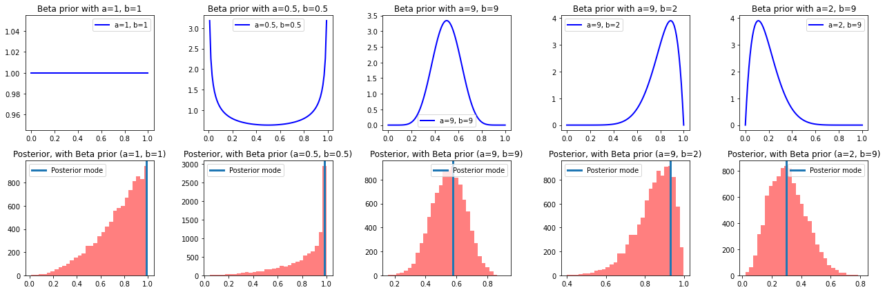
We model the number of likes \(Y_n\) received by the \(n\)-th movie as a binomial variable \(Y_n | \theta_n\sim Bin(R_n, \theta_n)\), we model our prior beliefs and uncertainty about \(\theta\) using a beta distribution \(\theta_n \sim Beta(\alpha, \beta)\).

Show code cell content

Hide code cell content

#A list of beta distribution shapes to try out
beta_shapes = [(1, 1), (0.5, 0.5), (9, 9), (9, 2), (2, 9)]
#Length of the list of shapes
n = len(beta_shapes)

#Get the name of the first movie in the top 25 list
movie_name = top_movies[0][0]

#Get the ratings info for the first movie in the top 25 list
likes = top_movies[0][1]
total_ratings = top_movies[0][2]
likability = top_movies[0][3]

#Number of samples to use when approximating our posterior
samples = 10000

print('{}: {} ({}/{})'.format(movie_name, likability, likes, total_ratings))
fig, ax = plt.subplots(2, n, figsize=(18, 6))
ax = plot_priors_with_posteriors(ax, beta_shapes, likes, total_ratings, samples)
plt.tight_layout()    
plt.show() 

French Twist (Gazon maudit) (1995): 1.0 (2.0/2.0)

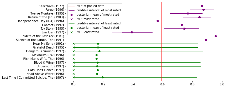
Credible Intervals for Movies with the Most and the Least Number of Ratings

Show code cell content

Hide code cell content

#paramters of our beta prior
a = 0.5
b = 0.5
#sort our list of movie info by like-percentage, in descending order
sorted_total_ratings = sorted(likability_list, key=lambda t: t[2], reverse=True)  

top_n = 10

##function to compute and plot the credible intervals for the movies with the most number of ratings
##and the movies with the least number of ratings
def plot_credible_intervals(a, b, ax):
    S = 1000
    movie_names = []
    for i in range(top_n):
        #compute the credible intervals of the movies with the most number of ratings
        post_samples = sample_posterior(a, b, sorted_total_ratings[i][1], sorted_total_ratings[i][2], S)
        ub = np.percentile(post_samples, 97.5)
        mean = np.percentile(post_samples, 50.0)
        lb = np.percentile(post_samples, 2.5)
        movie_names.append((top_n - (i + 1), sorted_total_ratings[i][0]))
        
        #plot the credible intervals
        if i == 0:
            ax.hlines(top_n - (i + 1), lb, ub, colors='purple', linewidth=1, label='credible interval of most rated')
            ax.scatter([mean], [top_n - (i + 1)], color='purple', label='posterior mean of most rated')
            ax.scatter([sorted_total_ratings[i][1] * 1. / sorted_total_ratings[i][2]], [top_n - (i + 1)], marker='x', color='purple', label='MLE most rated')
        else:
            ax.hlines(top_n - (i + 1), lb, ub, colors='purple', linewidth=1)
            ax.scatter([mean], [top_n - (i + 1)], color='purple')
            ax.scatter([sorted_total_ratings[i][1] * 1. / sorted_total_ratings[i][2]], [top_n - (i + 1)], marker='x', color='purple')
        
        #compute the credible intervals of the movies with the least number of ratings
        post_samples = sample_posterior(a, b, sorted_total_ratings[-(i + 1)][1], sorted_total_ratings[-(i + 1)][2], S)
        ub = np.percentile(post_samples, 97.5)
        mean = np.percentile(post_samples, 50.0)
        lb = np.percentile(post_samples, 2.5)
        movie_names.append((-top_n + i, sorted_total_ratings[-(i + 1)][0]))
        
        #plot the credible intervals
        if i == 0:
            ax.hlines(-top_n + i, lb, ub, colors='green', linewidth=1, label='credible interval of least rated')
            ax.scatter([mean], [-top_n + i], color='green', label='posterior mean of least rated')
            ax.scatter([sorted_total_ratings[-(i + 1)][1] * 1. / sorted_total_ratings[-(i + 1)][2]], [-top_n + i], marker='x', color='green', label='MLE least rated')
        else:
            ax.hlines(-top_n + i, lb, ub, colors='green', linewidth=1,)
            ax.scatter([mean], [-top_n + i], color='green')
            ax.scatter([sorted_total_ratings[-(i + 1)][1] * 1. / sorted_total_ratings[-(i + 1)][2]], [-top_n + i], marker='x', color='green')

            
        #compute the MLE of the pooled data
        total_likes = np.sum([rating[1] for rating in sorted_total_ratings])
        total_ratings = np.sum([rating[2] for rating in sorted_total_ratings])
            
        movie_names = sorted(movie_names, key=lambda x: x[0])
        
    ax.axvline(x=total_likes * 1. / total_ratings, color='red', label='MLE of pooled data')
    ax.legend(loc='best')
    ax.set_yticks(np.arange(-top_n, top_n + 1))
    ax.set_yticklabels([name[1] for name in movie_names])
    return ax

fig, ax = plt.subplots(1, 1, figsize=(10, 5))
ax = plot_credible_intervals(a, b, ax)
plt.show()

Empirical Bayes (ML-II) For the Beta-Binomial Model

Since the prior has a significant impact on the posterior when the number of ratings is small, we want to choose a prior that is appropriate for the data.

Idea: choose the hyperparameters \(\alpha, \beta\) for the beta prior such that the expected likelihood of the data, over \(\theta_n \sim Beta(\alpha, \beta)\), is maximized:

\[\begin{aligned} p(Y_1, \ldots, Y_N| \alpha, \beta) = \prod_{n=1}^N \int_0^1 Bin(Y_n|R_n, \theta_n) Beta(\theta_n|\alpha, \beta)d\theta_n = \prod_{n=1}^N {R_n \choose Y_n}\frac{B(\alpha + Y_n, \beta + R_n - Y_n)}{B(\alpha, \beta)} \end{aligned}\]

where \(B\) is the beta function. The marginal likelihood of the data \(p(Y_1, \ldots, Y_N| a, b)\) is called evidence.

This method of choosing the hyperparameters of the prior based on the data is called empirical Bayes or type-II maximum likelihood.

Question: doesn’t this violate the principle of choosing the prior independent of the data?

Method of Moments for Empirical Bayes (ML-II)

Since each marginal \(p(Y_n| \alpha, \beta)\) is a Beta-Binomial distribution, we know its first two moments:

\[\begin{split}\begin{aligned} \mathbb{E}\left[Y_n\right] &= R_n \frac{\alpha}{\alpha + \beta}\\ \text{Var}\left[Y_n\right] &= \frac{R_n \alpha\beta}{(\alpha + \beta)^2}\frac{\alpha + \beta + R_n}{\alpha + \beta + 1} \end{aligned}\end{split}\]

Now we can make the simplifying approximations that the \(Y_n\)’s are iid data from the same binomial, i.e. all have the same moments as above. Then we can use empirical moments to approximate the theoretical moments and solve for \(\alpha, \beta\):

\[\begin{split}\begin{aligned} \widehat{\mathbb{E}}\left[\frac{Y_n}{R_n}\right] &= \frac{\alpha}{\alpha + \beta}\\ \widehat{\text{Var}}\left[\frac{Y_n}{R_n}\right] &= \frac{\alpha\beta}{\overline{R}_n (\alpha + \beta)^2}\frac{\alpha + \beta + \overline{R}_n}{\alpha + \beta + 1} \end{aligned}\end{split}\]

where \(\widehat{\mathbb{E}}\) is sample mean and \(\widehat{\text{Var}}\) is sample variance and \(\overline{R}_n\) is the average total number of ratings.

Show code cell content

Hide code cell content

mean = np.mean([rating[1] * 1. / rating[2] for rating in sorted_total_ratings])
variance = np.std([rating[1] * 1. / rating[2]  for rating in sorted_total_ratings])**2
R_mean = np.mean([rating[2] for rating in sorted_total_ratings])

alpha_eb = 0.897869
beta_eb = 0.912247

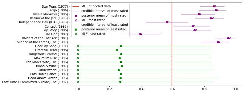
Empirical Bayes and Shrinkage

Computing the hyperparameters \(\alpha, \beta\) of the beta prior on \(\theta\) from the data, allows the ratings rich movies to influence the prior of ratings poor movies, since all movies contribute to the empirical Bayes estimate.

As a result, the estimates from ratings poor movies tend to shrink towards the population mean more so than ratings rich movies.

fig, ax = plt.subplots(1, 1, figsize=(10, 5))
ax = plot_credible_intervals(alpha_eb, beta_eb, ax)
plt.show()

13.3. Hierarchical Models and Empirical Bayes

A Hierarchical Model for Movie Rankings

We model the number of likes \(Y_n\) received by the \(n\)-th movie as a binomial variable \(Y_n|\theta_n\sim Bin(R_n, \theta_n)\), we model our prior beliefs and uncertainty about \(\theta\) using a beta distribution \(\theta_n \sim Beta(\alpha, \beta)\); finally, we model our uncertainty about \(\alpha, \beta\) using uniform distributions \(\alpha, \beta\sim U(0.5, 100)\):

\[\begin{split}\begin{aligned} \alpha, \beta &\sim U(0.5, 100)\\ \theta_n | \alpha, \beta &\sim Beta(\alpha, \beta)\\ Y_n|\theta_n &\sim Bin(R_n, \theta_n) \end{aligned}\end{split}\]

This is an example of a hierarchical model – a model with multiple layers of unknown variables.

There are overlaps between hierarchical models and latent variable models. Generally, we want the hierarchy in a hierarchical model to express scientifically meaningful conditional relationships. In latent variable models we want the latent variable to represent unknown aspects of the data rather than unknown parameters of our model.

Point Estimate Approximations of Inference in Hierarchical Models (MAP-II)

The posterior of the hierarchical model for movie ratings is \(p(\alpha, \beta, \theta_1, \ldots, \theta_N | Y_1, \ldots, Y_N)\), but since we know how \(\theta_n\) is conditioned on \(\alpha, \beta\), it is often easier to marginalize out \(\theta_n\) and work with \(p(\alpha, \beta |Y_1, \ldots, Y_N)\).

The central idea is that by inferring the posterior \(p(\alpha, \beta |Y_1, \ldots, Y_N)\), \(\alpha\) and \(\beta\) are influenced by the entire data set and thus ratings poor movies can borrow statistical strength from ratings rich movies through the way \(\theta_n\) depends on \(\alpha, \beta\).

However, performing full Bayesian inference on hierarchical models can be difficult. Thus, we can make a point estimate approximation of \(p(\alpha, \beta |Y_1, \ldots, Y_N)\):

\[\alpha^*, \beta^* = \text{argmax}_{\alpha, \beta} p(\alpha, \beta |Y_1, \ldots, Y_N).\]

When we perform the usual Bayesian inference on \(p(Y_n|\theta_n)p(\theta_n|\alpha^*, \beta^*)\), this is called the type-II MAP method.

But when \(\alpha, \beta\) are uniform random variables, the above becomes:

\[\alpha^*, \beta^* = \text{argmax}_{\alpha, \beta} p(Y_1, \ldots, Y_N |\alpha, \beta),\]

When we perform the usual Bayesian inference on \(p(Y_n|\theta_n)p(\theta_n|\alpha^*, \beta^*)\), this is just our empirical Bayes or type-II MLE method!

13.4. Summary

The questions we ask in this chapter are “When should we be Bayesian? How Bayesian should we be?”

Consider the kidney cancer data set from the Chapter 9 problem set: We posit that the observed number of cases of kidney cancer, \(y_j\), for the \(j\)-th county (with total population \(n_j\)) is a Poisson random variable that depends on the true underlying cancer rate, \(\theta\):

\[\begin{aligned} y_j | \theta_j &\sim Poisson(5 \cdot n_j \cdot \theta_j), \quad j = 1, \ldots, N \end{aligned}\]

1. (The MLE Model) Why not use MLE estimates of \(\theta\)? \( \theta_{\text{MLE}} = \frac{y_j}{n_j} \)

2. (The Bayesian Model) Why not use choose an arbitrary prior for \(\theta\) or choose a different prior per county?

\[\begin{split}\begin{aligned} y_j | \theta_j &\sim Poisson(5 \cdot n_j \cdot \theta_j), \quad j = 1, \ldots, N\\ \theta_j &\sim Gamma(\alpha, \beta), \quad j = 1, \ldots, N \end{aligned}\end{split}\]

3. (The Empirical Bayes Model) Why should we choose \(\alpha\), \(\beta\) using type-II MLE or empirical Bayes? Idea: choose the hyperparameters \(\alpha, \beta\) for the beta prior such that the evidence, is maximized:

\[\begin{aligned} \alpha_{\text{MLE-II}}, \beta_{\text{MLE-II}} = \text{argmax}_{\alpha, \beta} p(Y_1, \ldots, Y_N| \alpha, \beta) = \text{argmax}_{\alpha, \beta} \prod_{j=1}^J \int_0^1 Poisson(Y_j; 5 \cdot n_j \cdot \theta_j) Gamma(\theta_j; \alpha, \beta)d\theta_j \end{aligned}\]

4. (The Hierarchical Bayes Model) Why should we choose to use a hierarchical Bayes model?

\[\begin{split}\begin{aligned} y_j| \theta_j &\sim Poisson(5 \cdot n_j \cdot \theta_j), \quad j = 1, \ldots, N\\ \theta_j | \alpha, \beta &\sim Gamma(\alpha, \beta), \quad j = 1, \ldots, N\\ \alpha &\sim Gamma(a, b)\\ \beta &\sim Gamma(c, d) \end{aligned}\end{split}\]

5. (Broader Impact) Why should we care so much about which model to choose?

   • Which downstream decisions might be affected by the predictions of this model and how? So what if I underestimate cancer rates? So what if I overestimate?

   • Which counties are affected by the overfitting tendencies of MLE?

   • Which counties are affected by a poor choice of prior?

   • Who lives in these counties?

   • If your model negatively affects individual lives, would the negative effects be random or exacerbate systemic inequalities?
     
     

6. (The Small Data within Big Data Problem) The small data with big data problem is everywhere in machine learning. It might appear under names like “cohort imbalance”, “sampling bias”.

   • Health care: women, people of non-european descent, folks without insurance (and primary care) etc are extremely underrepresented

   • What can go wrong with modeling data with an underrepresented cohort?

     

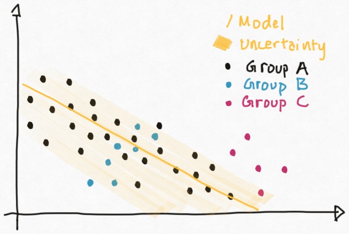
   • Why can’t you just collect more data?
     
     

7. (Why Should Engineers and ML Researchers Care About Broader Impact?) Is it your responsibility as an engineer to care about broader impact? To what extent is this your responsibility?

   • If you’re just an engineer in a long ML pipeline in an industry setting, how much should you care about broader impact? Don’t company have a legal and ethics department that handles all that?

   • If you’re just a in-house attorney or social scientist at a tech company, what properties of MLE, Bayesian, Empirical Bayes and Hierarchical Bayes models should you know?

13.5. Exercises

These problems were originally assigned as homework. Data files are in the book’s data/ folder. Worked solutions, where available, are collapsed beneath the questions they answer; try each problem before expanding them.

Problem Set: Modeling Kidney Cancer Data

In this problem, we will continue to work with the US Kidney Cancer Data set, kcancer.csv. This is a dataset of kidney cancer frequencies across the US over 5 years on a per county basis.

In this problem set, we focus on comparing different types of models for this data set.

Exercise: Part I: Empirical Bayes

Let \(N\) be the number of counties; let \(y_j\) the number of kidney cancer case for the \(j\)-th county, \(n_j\) the population of the \(j\)-county and \(\theta_j\) be the underlying kidney cancer rate for that county. The following is a Bayesian model for our data:

\[\begin{split}\begin{aligned} y_j | \theta_j &\sim Poisson(5 \cdot n_j \cdot \theta_j), \quad j = 1, \ldots, N\\ \theta_j &\sim Gamma(\alpha, \beta), \quad j = 1, \ldots, N \end{aligned}\end{split}\]

where \(\alpha, \beta\) are hyper-parameters of the model.

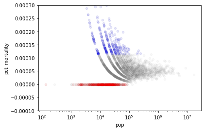
1. (Visualize the raw cancer rates) Produce a scatter plot of the raw cancer rates (pct mortality) vs the county population size (in log scale). Highlight the top 300 raw cancer rates in red. Highlight the bottom 300 raw cancer rates in blue. What can you say about the counties with the highest and lowest raw cancer rates.
   
   

2. (Empirical Bayes) Using Empirical Bayes and moment matching, choose values for the hyperparameters \(\alpha, \beta\) based on your data. Use these values of \(\alpha\) and \(\beta\) to obtain posterior distributions for each county.

Hint: You’ll first need to derive the fact that the evidence for a Poisson-Gamma model has a Negative Binomial distribution.

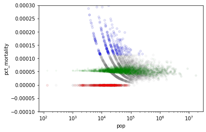
3. (Posterior Means) Produce a scatter plot of the raw cancer rates (pct mortality) vs the county population size (in log scale). Highlight the top 300 raw cancer rates in red. Highlight the bottom 300 raw cancer rates in blue. Finally, on the same plot again, scatter plot the posterior mean cancer rate estimates vs the county population size, highlight these means in green.

   Using the scatter plot, explain why using the posterior means (from our model) to estimate cancer rates is preferable to studying the raw rates themselves.

Solution: Part I, Question 1

# data_df is the dataframe of your data
# estimates is a numpy array of cancer rate estimates, one for each county
def scatter_plot_cancer_rates(data_df, estimates=None):
    ax = data_df.plot(kind='scatter', x="pop",y="pct_mortality", alpha=0.1, color="grey")
    bot_kcancer_counties = data_df.sort_values(by='pct_mortality',ascending=True)[:300]
    top_kcancer_counties = data_df.sort_values(by='pct_mortality',ascending=False)[:300]
    top_kcancer_counties.plot(kind='scatter',x="pop",y="pct_mortality",alpha=0.5, color="red", ax=ax, logx=True)
    bot_kcancer_counties.plot(kind='scatter',x="pop",y="pct_mortality",alpha=0.5, color="blue", ax=ax, logx=True)
    if estimates is not None:
        ax.plot(data_df['pop'], 5 * estimates, '.', alpha=0.2, color="green")
    ax.set_ylim([-0.0001, 0.0003])

df=pd.read_csv("../data/kcancer.csv")
y = df['dc'].values
n = df['pop'].values

scatter_plot_cancer_rates(df)
plt.show()

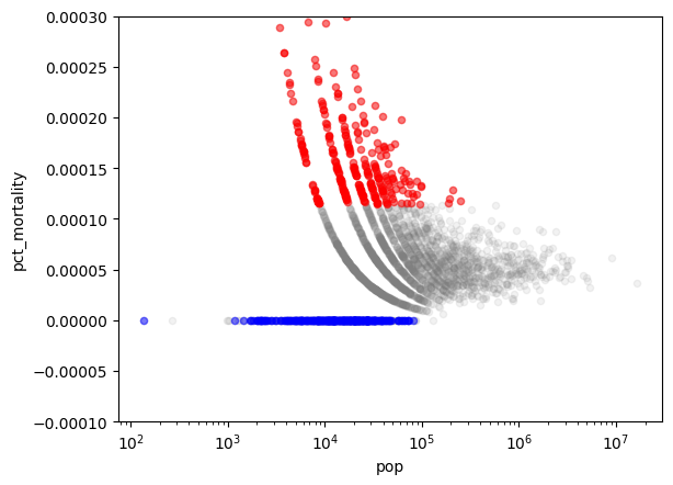
It looks like the counties with the highest and lowest raw cancer rates are also the counties with lower populations. This pattern indicates that the raw cancer rates (MLE estimates) may be overfitting to outliers in the data and the cancer rates of counties with fewer people are more exaggerated.

Solution: Part I, Question 2

We note that the Gamma-Poisson model is conjugate, that is, the posterior, posterior predictive and prior predictive all have closed forms. In particular, the posterior distribution is a Gamma distribution and the prior predictive is a Negative Binomial Distribution.

\[\begin{split}\begin{aligned} p(\theta_j | y_j) &\propto Poisson(y_j; 5 \cdot n_j \cdot \theta_j) Gamma(\theta_j; \alpha, \beta)\\ &\propto e^{-5 \cdot n_j \cdot \theta_j} \left(5 \cdot n_j \cdot \theta_j\right)^{y_j} \theta_j^{\alpha - 1} e^{-\beta\theta_j}\\ &= e^{-\left(5 \cdot n_j \cdot \theta_j + \beta\theta_j\right)} \theta_j^{\alpha + y_j - 1} \left(5 \cdot n_j\right)^{y_j}\\ &\propto e^{-\left(5 \cdot n_j + \beta\right)\theta_j} \theta_j^{\alpha + y_j - 1} \end{aligned}\end{split}\]

We see that \(p(\theta_j | y_j)\) is a Gamma distribution, \(Gamma(\alpha + y_j, 5 n_j + \beta)\).

Recall that the prior predictive, \(p(y_j)\), can computed by

\[ p(y_j) = \frac{p(y_j | \theta_j) p(\theta_j)}{p(\theta_j | y_j)}. \]

In our case, this becomes

\[\begin{split}\begin{aligned} p(y_j) &= \frac{Poisson(y_j; 5 \cdot n_j \cdot \theta_j) Gamma(\theta_j; \alpha, \beta)}{Gamma(\alpha + y_j, 5 n_j + \beta)}\\ &= \frac{\frac{\left(5 \cdot n_j \cdot \theta_j\right)^{y_j}}{y_j!} e^{-5 \cdot n_j \cdot \theta_j} \frac{\beta^\alpha}{\Gamma(\alpha)} \theta_j^{\alpha - 1} e^{-\beta\theta_j}}{\frac{\left(5 n_j + \beta\right)^{\left( \alpha + y_j\right)}}{\Gamma\left(\alpha + y_j\right)} \theta_j^{\alpha + y_j - 1} e^{-\left(5 n_j + \beta\right) \theta_j}}\\ &= \frac{\beta^\alpha\Gamma\left(\alpha + y_j\right) \left(5 \cdot n_j\right)^{y_j} \theta_j^{\alpha + y_j - 1}e^{-\left(5 \cdot n_j + \beta\right)\theta_j}}{y_j!\Gamma(\alpha) \left(5 n_j + \beta\right)^{\left( \alpha + y_j\right)}\theta_j^{\alpha + y_j - 1} e^{-\left(5 n_j + \beta\right) \theta_j}}\\ &= \frac{\beta^\alpha\Gamma\left(\alpha + y_j\right) \left(5 \cdot n_j\right)^{y_j}}{y_j!\Gamma(\alpha) \left(5 n_j + \beta\right)^{\left( \alpha + y_j\right)}}\\ &= \frac{\Gamma\left(\alpha + y_j\right)}{y_j!\Gamma(\alpha)}\frac{\beta^\alpha}{\left(5 n_j + \beta\right)^{\alpha}} \frac{\left(5 \cdot n_j\right)^{y_j}}{\left(5 n_j + \beta\right)^{y_j}}\\ &= \frac{\Gamma\left((\alpha + y_j - 1) + 1\right)}{y_j!\Gamma(\alpha)} \left( \frac{\beta}{5 n_j + \beta}\right)^\alpha \left( \frac{5 \cdot n_j}{5 n_j + \beta}\right)^{y_j}\\ &= \frac{(\alpha + y_j - 1)\Gamma\left((\alpha + y_j - 2) + 1\right)}{y_j!\Gamma(\alpha)} \left( \frac{\beta}{5 n_j + \beta}\right)^\alpha \left( \frac{5 \cdot n_j}{5 n_j + \beta}\right)^{y_j}\\ &\vdots\\ &= \frac{(\alpha + y_j - 1)!}{y_j!\Gamma(\alpha)}\left( \frac{\beta}{5 n_j + \beta}\right)^\alpha \left( \frac{5 \cdot n_j}{5 n_j + \beta}\right)^{y_j}\\ &= \frac{(\alpha + y_j - 1)!}{y_j!(\alpha - 1)!}\left( \frac{\beta}{5 n_j + \beta}\right)^\alpha \left( \frac{5 \cdot n_j}{5 n_j + \beta}\right)^{y_j}\\ &= \binom{\alpha + y_j - 1}{y_j}\left( \frac{\beta}{5 n_j + \beta}\right)^\alpha \left( \frac{5 \cdot n_j}{5 n_j + \beta}\right)^{y_j} \end{aligned}\end{split}\]

In the above, we’ve used the relation \(\Gamma(n + 1) = n\Gamma(n)\) to obtain:

\[\begin{split}\begin{aligned} \Gamma\left(\alpha + y_j\right) &= (\alpha + y_j - 1)!\\ \Gamma(\alpha) &= (\alpha - 1)! \end{aligned}\end{split}\]

Thus, \(p(y_j)\) can be parametrized as \(NegBin\left(\alpha, \frac{5 n_j}{5 n_j + \beta}\right)\). From this, we can compute the mean and variance of \(y_j\) as

\[\begin{split}\begin{aligned} \mathbb{E}[y_j] &= \frac{5 n_j \alpha }{\beta}\\ \mathrm{Var}[y_j]&= \frac{(5 n_j)^2\alpha}{\beta^2} + \frac{5 n_j\alpha}{\beta} \end{aligned}\end{split}\]

In Type-II MAP methods, typically, we choose a distribution involving the data and the hyperparameters, like the evidence, \(p(y_j | \alpha, \beta)\), or the joint distribution of the data and the hyperparameters, \(p(y_j, \alpha, \beta)\). We then seek values of \(\alpha\), \(\beta\) that maximizes the “likelihood” of the data given by these functions. Note that maximizing \(p(y_j | \alpha, \beta)\) and \(p(y_j, \alpha, \beta)\) may be difficult (especially when these functions have multiple local optima). Thus, another approach is to estimate \(\alpha\) and \(\beta\) by performing moment matching. That is, we set the expectation and variance of these distributions to values computed from the data; using these equations we can solve for \(\alpha\) and \(\beta\).

Unfortunately, obtaining an valid estimate of \(\mathbb{E}[y_j]\) (and \(\mathrm{Var}[y_j]\)) requires us to have multiple samples of \(y_j\), for a fixed \(j\), and to average them. Instead, what we have are samples from different \(y_j\)’s (each from a different distribution). If we are permitted to be a bit sloppy, we can treat the set of \(y_j\) values are samples from the same distribution. That is, we simply set

\[\begin{split}\begin{aligned} \bar{y}_j = \frac{1}{N}\sum^N_{j=1} y_j &= \mathbb{E}[y_j],\\ sample\_var[y_j]&= \mathrm{Var}[y_j]. \end{aligned}\end{split}\]

If we want to be more precise, we’d want to adjust the number of deaths, \(y_j\), in the \(j\)-th county, by the population of the county. That is, we set

\[\begin{split}\begin{aligned} \overline{\frac{y_j}{n_j}} = \frac{1}{N}\sum^N_{j=1} \frac{y_j}{n_j} &= \frac{5 \alpha }{\beta},\\ sample\_var\left[\frac{y_j}{n_j}\right]= \frac{25\alpha}{\beta^2} + \frac{5\alpha}{n_j\beta} &= \mathbb{E}\left[\frac{y_j}{n_j}\right] \left( \frac{5}{\beta} + \frac{1}{n_j}\right). \end{aligned}\end{split}\]

In order to make use of all of our data, we further substitute the empirical mean of the population, \(\bar{n}_j\), for \(n_j\).

adjusted_y = df['dc'] / df['pop']
y_mean = np.mean(adjusted_y)
y_var = np.var(adjusted_y)
pop_mean = np.mean(df['pop'])

print('empirical cancer population adjusted mean: ', y_mean)
print('empirical cancer population adjusted var: ', y_var)
print('empirical population mean: ', pop_mean)

empirical cancer population adjusted mean:  5.786552354108626e-05
empirical cancer population adjusted var:  2.527523010812238e-09
empirical population mean:  160512.41021522647

Substituting the empirical values into the two equations above, we get:

\[\begin{split}\begin{aligned} \mathtt{5.78655235411e-05}&= \frac{5\alpha }{\beta},\\ \mathtt{2.52752301081e-09}&= \mathtt{5.78655235411e-05}\left(\frac{5}{\beta} + \frac{1}{\mathtt{160512.410215}}\right). \end{aligned}\end{split}\]

Solving for \(\alpha, \beta\), we get

\[\begin{split}\begin{aligned} \alpha &= \frac{\mathtt{5.78655235411e-05}\cdot\beta}{5}\\ \beta &= \frac{5}{\frac{\mathtt{2.52752301081e-09}}{\mathtt{5.78655235411e-05}} - \frac{1}{\mathtt{160512.410215}}} \end{aligned}\end{split}\]

beta = 5. / (y_var / y_mean - 1. / pop_mean)
alpha = y_mean * beta / 5

print('alpha: ', alpha)
print('beta: ', beta)

alpha:  1.545173491879693
beta:  133514.17193888978

Since we already know the closed form of the posterior distribution, \(Gamma(\theta_j; \alpha + y_j, 5 n_j + \beta)\), we can directly compute the posterior mean or posterior mode estimate of \(\theta_j\). Or we can sample from \(Gamma(\alpha + y_j, 5 n_j + \beta)\) and compute the mean or mode from the samples:

post_samples = np.array([np.random.gamma(alpha + df['dc'].values, 1. / (beta + 5 * df['pop'].values)) for i in range(5000)])
theta_post_mean = np.mean(post_samples, axis=0)

Solution: Part I, Question 3

We can now plot the posterior mean estimate of the cancer death rate, \(\theta_j\) for each county along with the empirical cancer death rate:

scatter_plot_cancer_rates(df, estimates=theta_post_mean)
plt.show()

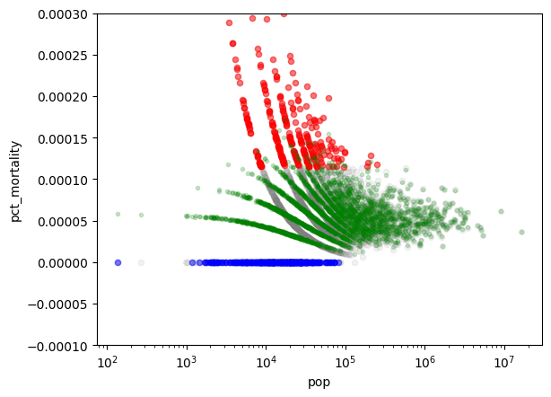
We see that the posterior mean estimates of cancer rates for counties with lower populations have shrunk towards the population average. The estimated rates for low-population counties using our Bayesian model are less extreme.

Exercise: Part II: Hierarchical Bayes

Rather than choosing fixed constants for the hyperparameters \(\alpha, \beta\), following the Bayesian philosophy, we typically put additional priors on quantities of which we are uncertain. That is, we model the kidney cancer rates using a hierarchical model:

\[\begin{split}\begin{aligned} y_j| \theta_j &\sim Poisson(5 \cdot n_j \cdot \theta_j), \quad j = 1, \ldots, N\\ \theta_j | \alpha, \beta &\sim Ga(\alpha, \beta), \quad j = 1, \ldots, N\\ \alpha &\sim Ga(a, b)\\ \beta &\sim Ga(c, d) \end{aligned}\end{split}\]

where \(a, b, c, d\) are hyperparameters.

1. (Posterior Marginal Means) Produce a scatter plot of the raw cancer rates (pct mortality) vs the county population size (in log scale). Highlight the top 300 raw cancer rates in red. Highlight the bottom 300 raw cancer rates in blue. Finally, on the same plot again, scatter plot the mean of the posterior marginal distribution over \(\theta_j\), i.e. \(p(\theta_j|y_1, \ldots, y_N)\), vs the county population size (in log scale), highlight these means in orange.

   You should use pymc3 to sample from the posterior. Compare pymc3’s sampler with your sampler from the Chapter 9 problem set, what is the difference (if any) in the performance of these samplers?
   
   

2. (Hierarchical Bayes vs Empirical Bayes) Compare the shrinkage of the posterior marginal means of the hierarchical model to the shrinkage of the posterior means from the Bayesian model with empirical Bayes estimates for \(\alpha, \beta\). What is the difference in shrinkage between the full hierarchical model and the Bayesian model with empirical Bayes?

Solution: Part II, Question 1

We implement the hierarchical model in pymc3!

import pymc3 as pm
from pymc3 import Model

#hyperparameters of hierarchical model
a=9
b=6
c=9
d=0.00001
 
#define hierarchical model in pymc3
with Model() as hiearchical_model:
    #hyperprior on alpha
    alpha = pm.Gamma('alpha', alpha=a, beta=b)
    #hyperprior on beta
    beta = pm.Gamma('beta', alpha=c, beta=d)
    #3,000 priors on theta
    theta = pm.Gamma('theta', alpha=alpha, beta=beta, shape=len(y))
    #convert rate into number of disease incidents
    mu = theta * 5 * n
    #likelihood
    y_obs = pm.Poisson('y', mu=mu, observed=y)

#sample 1000 samples from the posterior of the hierarchical model
#using 1000 iterations to tune the sampler
#the default sampler for pymc3 is the No-U-Turn Sampler (NUTS), a type of HMC
with hiearchical_model:
    trace = pm.sample(1000, tune=1000)

#defined burn-in
burn_in = .1
#define thinning
thin = 2
#select the county to visualize the traceplot for theta
county = 0

#plot the traceplots for one theta and alpha and beta
fig, ax = plt.subplots(1, 3, figsize=(30, 5))
N = len(trace['theta'].T[county])
theta_trace = trace['theta'][int(burn_in * N)::thin].T[county]
ax[0].plot(range(len(theta_trace)), theta_trace, color='gray', alpha=0.5)
ax[0].set_title('trace plot for theta_{}'.format(county))

alpha_trace = trace['alpha'][int(burn_in * N)::thin]
ax[1].plot(range(len(alpha_trace)), alpha_trace, color='green', alpha=0.5)
ax[1].set_title('trace plot for alpha')

beta_trace = trace['beta'][int(burn_in * N)::thin]
ax[2].plot(range(len(beta_trace)), beta_trace, color='purple', alpha=0.5)
ax[2].set_title('trace plot for beta')
plt.show()

It looks like that the chain for the posterior marginal of \(\theta_0\) has converged, and the chains for \(\alpha\) and \(\beta\) looks ok as well. Certainly, the traceplots of \(\alpha\) and \(\beta\) look much better here than for the Metropolis-Hastings-in-Gibbs sampler from the Chapter 9 problem set!

theta_samples = trace['theta'][int(burn_in * N)::thin].T
theta_post_mean_hier = np.mean(theta_samples, axis=1)

scatter_plot_cancer_rates(df, estimates=theta_post_mean_hier)
plt.show()

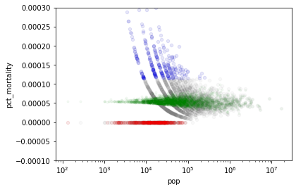
This plot is from the original pymc3 run (not re-run). It was drawn with the original plotting helper, which colours the top 300 raw rates blue and the bottom 300 red (the reverse of the question); the posterior means are in green.

Solution: Part II, Question 2

Plotting the posterior mean estimates of \(\theta_j\) from the hierarchical model, we see that the counties with least population shows the most amount of shrinkage! More so than in the case where we did Bayesian modeling with Empirical Bayes estimates of the prior \(\theta_j\).

This plot now tells us that the underlying cancer rates inferred from our model are similar across the country (all the rates are around 0.005%) with some random variations (i.e. some counties have higher rates and others have lower rates), but this variation is no longer correlated with population size.

This model of cancer rates is much better aligned with our scientific understanding of biological and environmental causes of cancer.

theta_samples = trace['theta'][int(burn_in * N)::thin].T
theta_post_mean_hier = np.mean(theta_samples, axis=1)

scatter_plot_cancer_rates(df, estimates=theta_post_mean_hier)
plt.show()

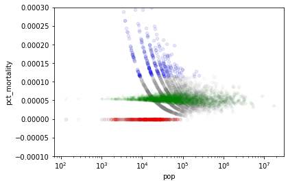
This plot is from the original pymc3 run (not re-run). It was drawn with the original plotting helper, which colours the top 300 raw rates blue and the bottom 300 red (the reverse of the question); the posterior means are in green.

Exercise: Part III: Broader Impact Analysis

Starting in 2020, major machine learning conferences are beginning to ask authors as well as reviewers to explicitly consider the broader impact of new machine learning methods. To properly evaluate the potential good or harm that a piece of technology (AI or not) can do to the general public, we need to be aware that no technology is deployed in ideal conditions or in perfectly neutral contexts. In order to assess the potential broader impact of technology, we need to analyze the social systems/institutions of which these technologies will become a part.

To help you analyze the broader impact of your technology, begin by considering the following questions:

I. Identify the relevant socio-technical systems

• In what social, political, economic system could the tech be deployed?

• How would the tech be used in these systems (what role will it take in the decision making processes)?
  
  

II. Identify the stakeholders

• Who are the users?

• Who are the affected communities (are these the users)?

  Hint: users are typically decision makers who will use the technology as decision aids (e.g. doctors), whereas affected communities may be folks who are impacted by these decisions but who are not represented in the decision making process (e.g. patients).
  
  

III. What types of harm can this tech do?

• What kinds of failures can this tech have?

• What kinds of direct harm can these failures cause?

• What kinds of harm can the socio-technical system cause?

  Hint: many technical innovations have niche applications, they may sit in a long chain of decision making in a complex system. As such, it may seem, at first glance, that these technologies have no immediate real-life impact. In these cases, it’s helpful to think about the impact of the entire system and then think about how the proposed innovations aid, hamper or change the goals or outcomes of this system.
  
  

IV. What types of good can this tech do?

• What kinds of needs do these users/communities have?

• What kinds of constraints do these users/communities have?
  
  

1. (Computational Footprint) In the Chapter 9 problem set, we considered the broader impact of the this hierarchical model for kidney cancer: we examined under what circumstances a hierarchical model for kidney cancer is more preferable to a MLE model or a Bayesian model with hand-picked priors. In this problem, we compare hierarchical Bayes and empirical Bayes.

   In practical terms, what are the real-life advantages and drawbacks of implementing an empirical Bayesian model compared with an hierarchical Bayesian model?

   Hint: for example, compare how tractable it is to implement the inference algorithm for each model, compare how easy it is to for the inference method for each model to converge (would you know that your training has converged?). Consider also: how easily could a practitioner diagnose the training process and how could they evaluate the model fit and what kinds of computational resources would be required to train each model.

2. (Mitigation of Potential Negative Impacts) Based on your answers for the previous question and your broader impact analysis from the Chapter 9 problem set, what information would the model designer/engineer need to disclose to the end-users to mitigate potentially negative impacts?

   Hint: consider how your end-user would be able to validate the model (how would they know if the model is working or has ceased to work once it has been deployed), how should the end-user choose between implementing a hierarchical Bayesian model or an empirical Bayesian model, how could the end-user identify and mitigate negative impacts (if they occur).

13.6. Further Reading

Hierarchical Bayes and Model Selection

• (Introductory) Visual explanation for why we do hierarchical modeling

• (In-Depth) Introduction to Hierarchical Models

• (Introductory) Taming False Discoveries with Empirical Bayes

• (Introductory) Bayesian Model Selection

• (Advanced) Model Selection with AIC, BIC etc

• (In-Depth) Understanding predictive information criteria for Bayesian models