Lab 5: KL-Divergence and Modeling with pymc3

This lab is adapted from AM207 (Harvard). Data files are in the book’s data/ folder. Worked solutions are collapsed: try each exercise before expanding them.

In this lab

1. The Benefits and Draw Backs of Variational Inference with KL-Divergence

2. Statistical Modeling with pymc3

Show code cell content

Hide code cell content

### Import basic libraries
import numpy as np
import pandas as pd
import sklearn as sk
from sklearn.linear_model import LinearRegression
import matplotlib.pyplot as plt
from pymc3 import model_to_graphviz, Model
import pymc3 as pm
%matplotlib inline

Closed Form KL-divergence for Two Gaussians

Let the target distribution be a bivariate Gaussian \(p(x) = \mathcal{N}(\mu_p, \Sigma_p)\), and let our variational family be isotropic bivariate Gaussians,

\[Q = \{\mathcal{N}(\mu_q, \sigma^2_q I_{2\times 2}) \,|\, \sigma^2_q > 0, \mu_q\in \mathbb{R}^2\}.\]

A bit of matrix algebra allows us to write the KL-divergence between two Gaussians as

\[ D_{\text{KL}}[\mathcal{N}(\mu_1, \Sigma_1) \| \mathcal{N}(\mu_2, \Sigma_2)] = \frac{1}{2} \left[ \log\frac{|\Sigma_2|}{|\Sigma_1|} - D + \text{tr}\left\{ \Sigma_2^{-1} \Sigma_1\right\} + (\mu_2 - \mu_1)^\top \Sigma_2^{-1}(\mu_2 - \mu_1) \right] \]

where \(D\) is the dimension of the two Gaussians.

Forward vs Reverse KL

When we fit an isotropic Gaussian \(\mathcal{N}(\mu_q, \Sigma_q)\) to a non-isotropic target Gaussian \(\mathcal{N}(\mu_p, \Sigma_p)\) using the KL-divergence, we mean to find

\[ \mu^*_q, \Sigma^*_q = \underset{\mu_q, \Sigma_q}{\text{argmin}} D_{\text{KL}}[\mathcal{N}(\mu_q, \Sigma_q) \| \mathcal{N}(\mu_p, \Sigma_p)] \]

This is often called minimizing the reverse KL-divergence. We can analytically solve this optimization problem, when we do, we get that

\[\begin{split}\begin{aligned} \mu^*_q &= \mu_p\\ (\Sigma^*_q)_{ii} &= \frac{1}{(\Sigma_p^{-1})_{ii}} \end{aligned}\end{split}\]

But remember that choosing to minimize KL-divergence when we approximate \(\mathcal{N}(\mu_p, \Sigma_p)\) is arbitrary. That is, we could have chosen another divergence measure. In particular, we could have chosen to minimize the forward KL-divergence:

\[ \mu^*_q, \Sigma^*_q = \underset{\mu_q, \Sigma_q}{\text{argmin}} D_{\text{KL}}[\mathcal{N}(\mu_p, \Sigma_p)\|\mathcal{N}(\mu_q, \Sigma_q)] \]

Analytically solve the above optimization problem gives us

\[\begin{split}\begin{aligned} \mu^*_q &= \mu_p\\ (\Sigma_q)_{ii} &= (\Sigma_p)_{ii} \end{aligned}\end{split}\]

Which KL-Divergence Should We Optimize?

Is there any difference in minimizing these two different divergences? That is, does the following hold?

\[ \underset{\mu_q, \Sigma_q}{\text{argmin}} D_{\text{KL}}[\mathcal{N}(\mu_q, \Sigma_q) \| \mathcal{N}(\mu_p, \Sigma_p)] \overset{?}{=} \underset{\mu_q, \Sigma_q}{\text{argmin}} D_{\text{KL}}[\mathcal{N}(\mu_p, \Sigma_p)\|\mathcal{N}(\mu_q, \Sigma_q)] \]

If not, which type of KL-divergence should we use when fitting an isotropic Gaussian \(\mathcal{N}(\mu_q, \Sigma_q)\) to a non-isotropic target Gaussian \(\mathcal{N}(\mu_p, \Sigma_p)\)?

Solution

import scipy as sp
import scipy.stats

# functions to compute the optimal variational distribution under reverse and forward KL
reverse_kl = lambda mu_p, Sigma_p: (mu_p, np.diag(np.diag(np.linalg.inv(Sigma_p))**-1))
forward_kl = lambda mu_p, Sigma_p: (mu_p, np.diag(np.diag(Sigma_p)))

#mean of the multivariate Gaussian
mu_p = [120, 4]
#covariance matrix of the multivariate Gaussian
Sigma_p = 10 * np.ones((2, 2)) + 2 * np.eye(2)
#optimal variational distribution using KL-divergence
mu_q, Sigma_q = reverse_kl(mu_p, Sigma_p)
#optimal variational distribution using forward KL-divergence
mu_q_forward, Sigma_q_forward = forward_kl(mu_p, Sigma_p)

#define points that include most of the probability mass of the pdf
x, y = np.mgrid[112:128:.01, -4:11:.01]
pos = np.dstack((x, y))
#get the value of the target pdf at those points
z_p = sp.stats.multivariate_normal(mu_p, Sigma_p).pdf(pos)
#get the value of the variational pdf at those points
z_q = sp.stats.multivariate_normal(mu_q, Sigma_q).pdf(pos)
z_q_forward = sp.stats.multivariate_normal(mu_q_forward, Sigma_q_forward).pdf(pos)

#plot the target density against variational densities
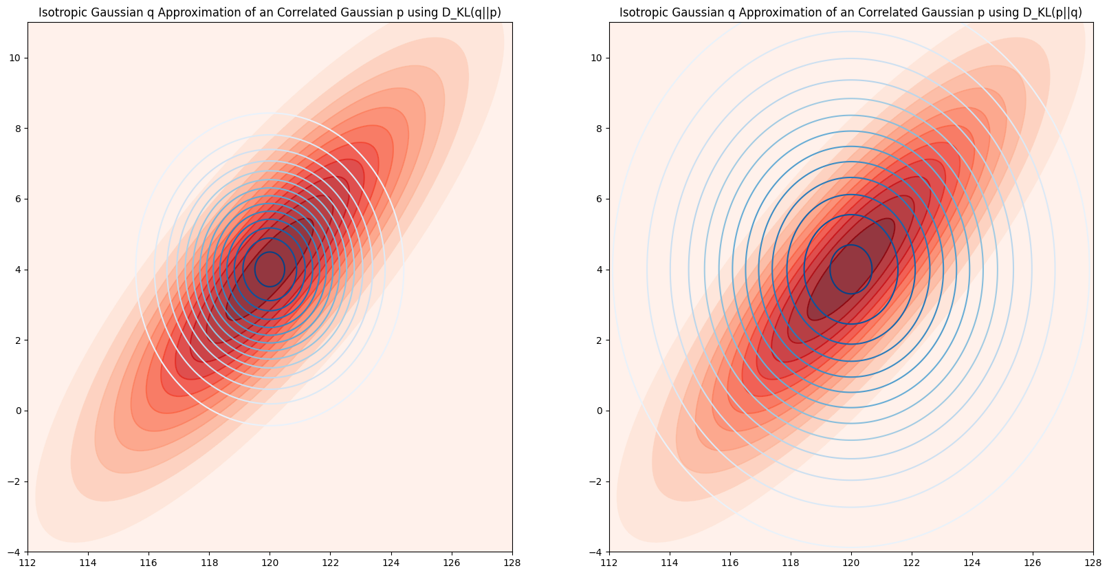
fig, ax = plt.subplots(1, 2, figsize=(20, 10))
#variational approximation using KL
ax[0].contourf(x, y, z_p, levels=14, cmap='Reds', alpha=0.8)
ax[0].contour(x, y, z_p, levels=14, cmap='Reds', alpha=0.8)
ax[0].contour(x, y, z_q, levels=14, cmap='Blues', alpha=1.)
ax[0].set_title('Isotropic Gaussian q Approximation of an Correlated Gaussian p using D_KL(q||p)')
ax[0].set_xlim([112, 128])
ax[0].set_ylim([-4, 11])
#variational approximation using forward KL
ax[1].contourf(x, y, z_p, levels=14, cmap='Reds', alpha=0.8)
ax[1].contour(x, y, z_p, levels=14, cmap='Reds', alpha=0.8)
ax[1].contour(x, y, z_q_forward, levels=14, cmap='Blues', alpha=1.)
ax[1].set_title('Isotropic Gaussian q Approximation of an Correlated Gaussian p using D_KL(p||q)')
ax[1].set_xlim([112, 128])
ax[1].set_ylim([-4, 11])
plt.show()

S = 4000
#get samples from the target distribution
p_samples = np.random.multivariate_normal(mu_p, Sigma_p, size=S)
#get samples from the variational distribution
q_samples = np.random.multivariate_normal(mu_q, Sigma_q, size=S)
q_forward_samples = np.random.multivariate_normal(mu_q_forward, Sigma_q_forward, size=S)

x_min = np.min((p_samples[:, 0].min(), q_samples[:, 0].min(), q_forward_samples[:, 0].min()))
x_max = np.max((p_samples[:, 0].max(), q_samples[:, 0].max(), q_forward_samples[:, 0].max()))

y_min = np.min((p_samples[:, 1].min(), q_samples[:, 1].min(), q_forward_samples[:, 1].min()))
y_max = np.max((p_samples[:, 1].max(), q_samples[:, 1].max(), q_forward_samples[:, 1].max()))

#plot the marginals of the target and the variational distributions
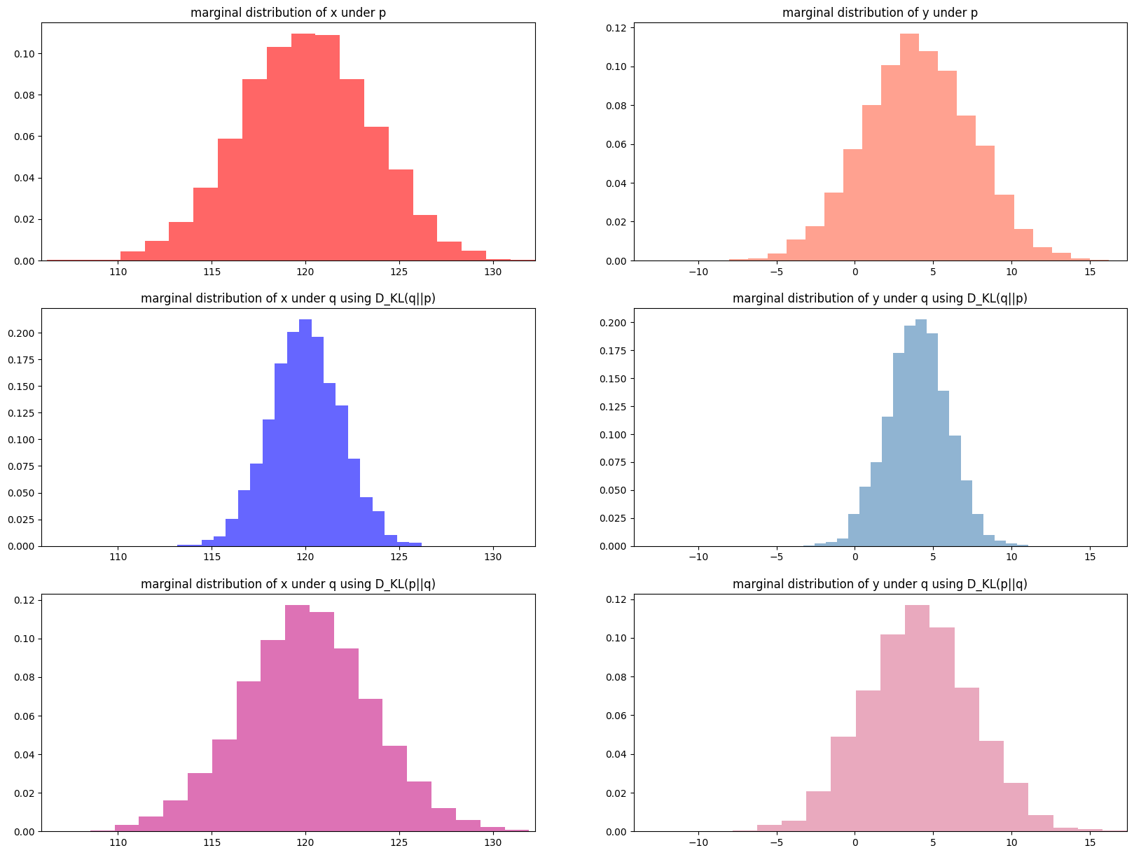
fig, ax = plt.subplots(3, 2, figsize=(20, 15))
ax[0, 0].hist(p_samples[:, 0], bins=20, density=True, color='red', alpha=0.6)
ax[0, 0].set_title('marginal distribution of x under p')
ax[0, 0].set_xlim([x_min, x_max])

ax[0, 1].hist(p_samples[:, 1], bins=20, density=True, color='tomato', alpha=0.6)
ax[0, 1].set_title('marginal distribution of y under p')
ax[0, 1].set_xlim([y_min, y_max])

ax[1, 0].hist(q_samples[:, 0], bins=20, density=True, color='blue', alpha=0.6)
ax[1, 0].set_xlim([x_min, x_max])
ax[1, 0].set_title('marginal distribution of x under q using D_KL(q||p)')

ax[1, 1].hist(q_samples[:, 1], bins=20, density=True, color='steelblue', alpha=0.6)
ax[1, 1].set_xlim([y_min, y_max])
ax[1, 1].set_title('marginal distribution of y under q using D_KL(q||p)')


ax[2, 0].hist(q_forward_samples[:, 0], bins=20, density=True, color='mediumvioletred', alpha=0.6)
ax[2, 0].set_xlim([x_min, x_max])
ax[2, 0].set_title('marginal distribution of x under q using D_KL(p||q)')

ax[2, 1].hist(q_forward_samples[:, 1], bins=20, density=True, color='palevioletred', alpha=0.6)
ax[2, 1].set_xlim([y_min, y_max])
ax[2, 1].set_title('marginal distribution of y under q using D_KL(p||q)')
plt.show()

Not covered here: a written answer to which KL-divergence to use.

pymc3

Introduction to pymc3

pymc3 is a python package for building and performing inference on Bayesian statistical models. Notably, pymc3 implements a number of popular approximate inference methods like Markov chain Monte Carlo (MCMC) and variational inference (VI).

Along with core model specification and fitting functionality, PyMC3 includes functionality for summarizing output and for model diagnostics.

Defining a Basic Model in pymc3

After importing the library and instantiating a pymc3 model:

import pymc3 as pm
bayesian_model = pm.Model()

We defined our model using a context manager (with statement – a python construct that manages the allocate and release resources involved with performing an action).

#define hierarchical model in pymc3
with Model() as bayesian_model:
    #priors on theta
    theta = pm.Gamma('theta', alpha=alpha, beta=beta)
    #convert rate into number of disease incidents
    mu = theta * 5 * average_pop
    #likelihood
    y_obs = pm.Poisson('y', mu=mu, observed=y)

The model is specified declaratively inside the context manager.

A Pooled Bayesian Model for the Kidney Cancer Data Set

Suppose we treat all the cancer incidents \(y_j\) across the US as iid samples from a single Poisson distribution \(y_j \sim Poi(\theta)\), where \(\theta\) is the same underlying rate for kidney cancer for every county.

Question: Is this a good way to model the Kidney cancer data?

df=pd.read_csv("../data/kcancer.csv")
y = df['dc'].values
n = df['pop'].values
average_pop = n.mean()

#hyperparameters of Bayesian model
alpha=10.
beta=1000.
 
#define hierarchical model in pymc3
with Model() as bayesian_model:
    #priors on theta
    theta = pm.Gamma('theta', alpha=alpha, beta=beta)
    #convert rate into number of disease incidents
    mu = theta * 5 * average_pop
    #likelihood
    y_obs = pm.Poisson('y', mu=mu, observed=y)

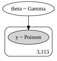
#draw graphical model for the thing we just defined  
model_to_graphviz(bayesian_model)

Inference Using pymc3

A number of different samplers are implemented in pymc3. You have the flexibility of specifying different samplers for different variables in your model (e.g. you can implement a MH-in-Gibbs sampler using pymc3).

#sample 1000 samples from the posterior of the model, using 1000 iterations to tune the sampler
#the default sampler for pymc3 is the No-U-Turn Sampler (NUTS), a type of HMC
with bayesian_model:
    #specifying a specific sampler
    steps = pm.Metropolis(vars=[theta, mu])
    #use the specify sampler to sample from the posterior of the model
    trace = pm.sample(1000,step=steps, tune=1000)
    #using default sampler
#     trace = pm.sample(1000, tune=1000)

Multiprocess sampling (2 chains in 2 jobs)
Metropolis: [theta]
Sampling 2 chains: 100%|██████████| 4000/4000 [00:00<00:00, 9235.06draws/s]
The number of effective samples is smaller than 25% for some parameters.

Diagnostics Using pymc3

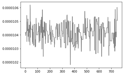
pymc3 implements also a large number of convergence diagnostics for MCMC samplers – traceplots, auto-correlation plots, Gelman-Rubin statistic etc.

posterior_samples = trace['theta'][500::2]
plt.plot(np.arange(len(posterior_samples)), posterior_samples, color='gray')
plt.show()

Posterior Predictive Sampling with pymc3

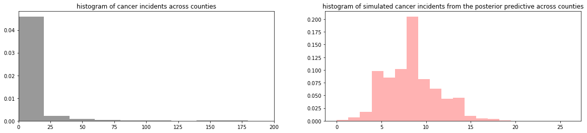
Given the trace and the model, pymc3 can also automatically sample from the posterior predictive.

pp_samples = pm.sample_posterior_predictive(trace, samples=1000, model=bayesian_model)
fig, ax = plt.subplots(1, 2, figsize=(20, 4))
ax[0].hist(y, bins=30, density=True, color='gray', alpha=0.8)
ax[0].set_xlim([0, 200])
ax[0].set_title('histogram of cancer incidents across counties')
ax[1].hist(pp_samples['y'].flatten(), bins=20, density=True, color='red', alpha=0.3)
ax[1].set_title('histogram of simulated cancer incidents from the posterior predictive across counties')
plt.show()

100%|██████████| 1000/1000 [00:00<00:00, 1153.18it/s]