What's in the Air? Using Mathematical Models to Predict Boston Air Quality

Team Members: Anthony DePinho*, Tara Ippolito*, Biyonka Liang*, Kaela Nelson*, Annamira O’Toole*

Postdoc Advisor: Weiwei Pan

Sponsors: Gary Adamkiewicz, Jaime Hart, Pavlos Protopapas

Code Repository

Interface

Table of Contents:

I. Abstract

II. Intro

III. Problem Statement and Methods

IV. Procedures and Methods

V. Mathematical Modeling

VI. Analysis

VII. Conclusion

VIII. Acknowledgements

IX. References

I. Abstract

Exposure to pollutants such as NO2, SO2, and PM2.5 are a significant concern, especially for those living in large cities. However, most major cities have five or fewer active air quality sensors. Various studies have shown that geostatistical models using traffic count, elevation, and land cover as variables can predict pollutant levels with high accuracy. Collecting training data containing sufficient geospatial variation often involves large scale deployment of sensors over the area of interest. In this study, we trained geospatial and spatio-temproal models for three EPA criteria pollutants - NO2, SO2, and PM2.5 - using data collected from 398 counties across the US and applied the models to produce intra-urban pollution concentration levels for a 107.495 square mile region covering the Greater Boston area. The performance of our geospatial model (Land Use Regression) and spatio-temporal model (Guassian Process) were comparable of similar models in literature. Our study also addresses the public health challenge of effectively and meaningfully communicating scientific findings in environmental science to the general public. Specifically, we designed an interactive web interface for visualizing our Boston air pollution predictions. This interface serves as a proof-of-concept for an accessible, educational, and scientific tool.

II. Introduction

Air pollutants originate from multiple sources, some anthropogenic and others from reactions in the atmosphere itself. Criteria pollutants are those whose levels are monitored and regulated by the EPA. These pollutants are amongst those that can significantly impact the environment and on human health. For example, Particulate Matter 2.5 (PM2.5) is an especially dangerous pollutant in long-term human exposure. Findings from the American Heart Association indicate that PM2.5 air pollution contributes to worsened cardiovascular health and (to a lesser extent) pulmonary health [3,7]. Stroke and arrhythmia, as well as heart failure exacerbation are some of the more serious consequences of exposure in individuals with heightened risk of cardiovascular problems. Currently, PM2.5 exposure is ranked as the 13th leading cause of worldwide mortality with approximately of 800,000 premature deaths per year [3]. Both NO2 and SO2 are particularly harmful for those with respiratory illnesses, they can also contribute to particulate matter concentration when they react with other chemicals in the atmosphere [8,9]. Literature suggests that NO2 and SO2 also impact cardiovascular health, especially in conjunction with particulate matter [7]. The Environmental Protection Agency reported that multiple studies showed evidence of increased risk of susceptibility to both viral and bacterial infections after NO2 exposures [9]. The same EPA report stated that airway inflammation and hyperresponsiveness were seen in human clinical studies [9]. The EPA report on SO2 exposure finds that studies indicate that SO2 is associated with episodic respiratory illness and aggravation of respiratory diseases [8]. Based on widespread assessment and study of the dangers of these pollutants, modeling their concentrations and educating the public is vital to improve human health.

Main sources of particulate matter are combustion of fossil fuels (i.e. traffic and power plants) [3], construction and demolition leading to particle suspension, as well as physiochemical transformation of gases already existing in the atmosphere [4]. The main sources of NO2 are the combustion of fossil fuels in industrial processes as well as from traffic [4]. SO2 concentration is mostly affected by combustion of fossil fuels that contain sulfur, this can be from cars as well as power plants [4].

III. Problem Statement and Methods

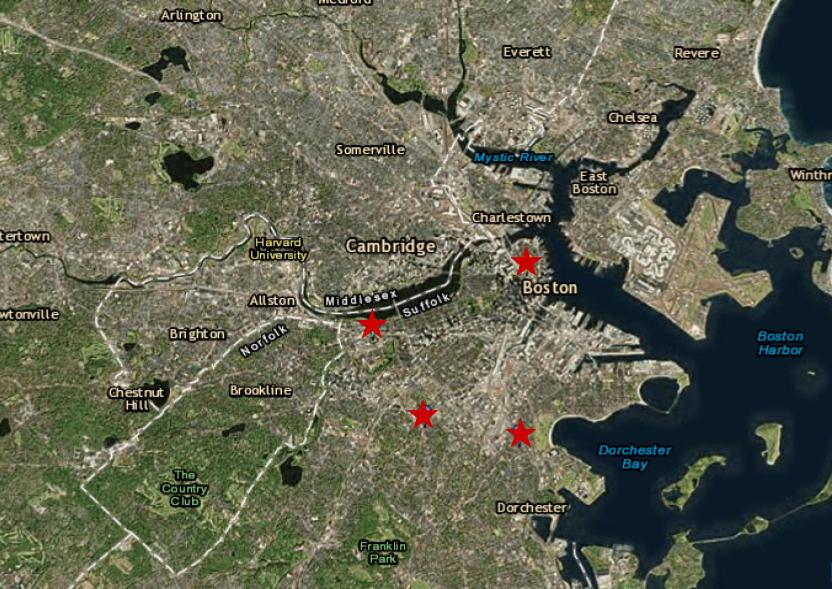
Fig 1. - Locations of EPA Air Quality Sensors in Greater Boston

There are two main challenges that motivate this project. Firstly, there are four Environmental Protection Agency (EPA) air quality sensors located in the Greater Boston area that are responsible for recording all air quality data for all the significant pollutants in the entire city (Figure 1). As large portions of the city are outside the range of existing sensors, there are insufficient EPA sensors to provide an adequate assessment of intra-urban spatial variations in air quality conditions. Since the installation of new sensors to provide more widespread coverage of land is a difficult task, our main objective is to implement statistical modeling techniques to model air pollution in areas that existing sensors do not cover. The independent variables impacting pollutant concentration that we will consider include land use and weather.

Another challenge that this project addresses is the difficulty of making scientific data and findings accessible to the general public, especially when such information affects the health and welfare of urban residents. While environmental monitoring organizations like the EPA makes all of its air quality data publicly available, this data consists of numerical databases or scientific reports. In these formats, the air quality information can be of limited use to laymen with little scientific training. Furthermore, air pollution data are often collected and reported by agencies for regulation purposes, not for health or educational purposes, thus there is a further gap to be filled connecting the results of air quality monitoring to public health concerns. A major goal of this project is to design an easy-to-read, interactive interface which provides a more intuitive visualization of Boston’s air quality. The interface will provide users with a way to understand air quality conditions on both a city wide and granular level. Our design for the interface aims to communicate the results of our statistical models meaningfully to anyone who uses the interface. In the end, we hope that our interface serves as an educational tool for the public, as a tool for scientists, and potentially as an aid in city policy and zoning decisions.

IV. Procedures and Methods

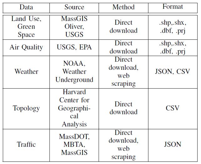
A. Data Collection

In our models, we include static geospatial data as well as dynamic data. Geospatial data consists of land use, topography and bus routes while dynamic data consists of traffic and weather.

Air quality from the four Boston sensor sites were collected hourly over several weeks. Our land use data was downloaded as GIS shapefiles, wherein the areas used for the training, testing and forecasting are covered by polygons (and multigons - nested polygons) each described by a single land use type. Average daily traffic volume and real-time traffic volume data was downloaded by state as point-wise estimates, i.e. reported for a network of sensor locations across each state. Elevations (sea level) are provided by Google Maps. Weather data was provided by the EPA for each sensor location. In addition, real-time weather data for stations throughout Boston was collected for a period of one week.

The training data consists of the above data collected from 398 counties throughout 16 US states, the majority of which where located on the East Coast. The trained models were applied to a 107.495 square mile region overing Greater Boston. This area was divided into a 50 by 50 grid (Figure 3). The grid cells are uniformly sized squares with a length of approximately one sixteenth of a square mile. The process in which we extracted geospatial predictors per grid cell is described in greater detail in the below section. All data sources and formats are shown in Figure I.

B. Data Rastering

Fig 2. - Distribution of Land Use in Site Data

Within each grid cell of our 50x50 Boston grid, we uniformly sampled 100 random points. Each point is assigned a land use type corresponding to the land use polygon within which it fell. The land use types of the sampled points within each cell are then categorized into 11 land use categories and totaled for each category producing a land use proportion or percentage break down for each grid cell. The distribution of land use types in our data is visualized in Figure 2. Next, the elevation is measured at each sampled point and the elevations are averaged to produce an average elevation per grid cell. Then, counts from traffic sensors falling within each grid are averaged producing a single indicator per cell. Finally, for the centroid of each cell, the data from the nearest five weather data are averaged.

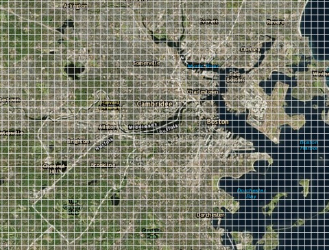
In the training set, 100 random points were uniformly sampled from a 1/16 squared mile grid centered at each EPA sensor site. Geospatial descriptors were extracted for each site through the same process as described above, with the exception that weather data was taken from EPA provided yearly averages rather than real-time data and for sites where this data was missing, we imputed the missing value with the average value for the state to which the site belonged. The land use data used to characterize the EPA sites in training set were collected by the US Geological Survey during the period from 1970 to 1980.

Fig 3. - Visual representation of Greater Boston Area grid system

The training data consists of data from 1,948 EPA monitoring sites in counties across 16 US states. The data was collected and averaged over the year of 1980. Because each site monitors different conditions and pollutants, we created subset datasets for each pollutant. We first subset out the sites that monitored our pollutants of interest: NO2, SO2 and PM2.5. The component PM2.5 readings (Silicon PM2.5, Titanium PM2.5, etc) were added for each site to obtain an overall PM2.5 reading for each site. The training set contains PM2.5 had 1949 observations, 311 NO2 and 585 SO2 observations.

C. Computational Resources

Our primary computing environment is Jupyter Notebook, using an IPython3 kernel. For statistical modeling we used SciPy and scikit-learn libraries, and we used Matplotlib for visualization. For manipulating GIS data, we use the Shapely and PyShp libraries. The web application is developed in D3, Leaflet, CSS, and HTML. Amazon Web Services is used for large scale data collection and processing. Finally, GitHub is used for project collaboration and organization.

V. Mathematical Modeling

A. Land Use Regression

Land Use Regression (LUR) is a linear regression model commonly used to predict air pollutant concentration based on geospatial variation, using predictors such as land use and average (static) weather conditions like wind speed and air pressure. A separate land use regression model was fit for each EPA criteria pollutant in our study. Our LUR model was trained and tested on data collected from US sites outside of Boston and, thereafter, used to predict concentration levels for each grid cell covering the Greater Boston Area. In addition, We performed variable selection and analysis to reason about the impact of dynamic variables on the concentration of atmospheric pollutants. The form of our LUR models is as follows

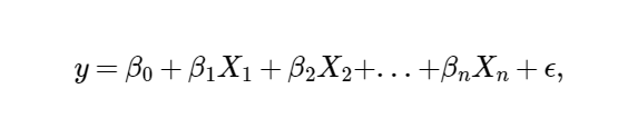
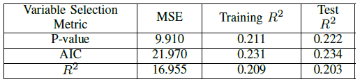
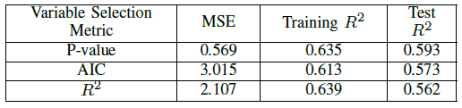
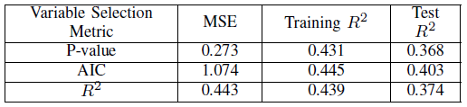
where the dependent variable y is the pollutant concentration of a given area; and X1...Xn represent the set or subset of geospatial predictor variables. Prior to variable selection, these predictors consist of a total of 14 variables from two categories: land use and weather. Land use types were categorized into industrial, commercial, medium density residential area, open space, crop land, water, wetland, transitional, forest, transportation, and urban public space. The weather data consists of 3 metrics: outdoor temperature, solar radiation and wind speed. These metrics were chosen as they were collected at the most sites that also collected our pollutants of interest.

B. Variable Selection and Cross Validation for LUR

Three different metrics were used for variable selection: p-value, R2 and AIC and the results compared. For R2 variable selection, 8-fold cross validation was implemented. Using backwards stepwise elimination, the set of predictor variables from the model with the worst metric (highest mean p-value, the lowest validation R2 and the highest AIC) was eliminated at each step. For all metrics, variable selection reduced the predictor set to 8-12 variables. Figures II through detail the results of our variable selection on all three LUR models. Testing R2 was in the range 0.203-0.234 for PM2.5, 0.562-0.593 for NO2 and 0.368-0.403 for SO2. By these metrics, we believe that levels of NO2 are most correlated with geospatial variations.

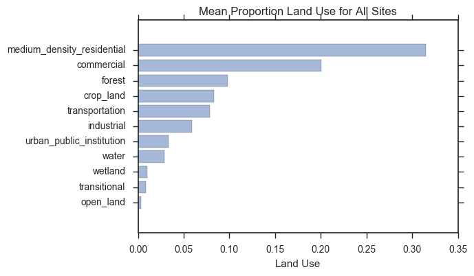
Using results from our variable selection, we analyzed predictors that appear most often in the final subsets (Figure 4).

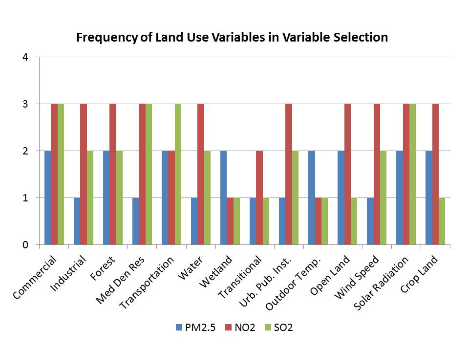
Fig 4. - Land use type frequency in variable selection

Since a primary source of all three pollutants is the combustion of fossil fuel, we expected to see certain land use variables, such as ”industrial”, ”transportation”, ”commercial” and ”medium density residential”, to be preserved by variable selection. The is validated by our variable selection results. However, in the selected subsets, we often observe variables that do not have known scientific relationships to the pollutants. ”Wetlands” for PM2.5 is one example. We suspect these unexpected inclusions may be the result of unknown confounding variables.

C. Gaussian Processes

Though LUR models are effective when we suspect strong correlation between geospatial variation and concentration levels of pollution, they lack flexibility to describe more complex (nonlinear) relationships between geospatial predictors and pollution levels. In addition, such models cannot be naturally extended to include dynamic (temporal) data. Thus, one way to introduce non-linearity and temporal dependence into our model is by the use of a Gaussian Process model. A Gaussian Process model is a statistical model that uses a nonparametric representation of the underlying function relating predictor and response. Specifically, we assume that any subset of our pollution concentration levels (both observed, y, and unknown, y*) have a joint Gaussian distribution,

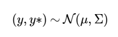
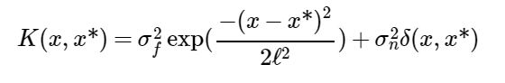
wherein the covariance matrix is determined by some metric of similarity of the geospatial and dynamic characteristics of the locations of the corresponding observation sites. That is, each entry in the covariance matrix is computed by a function in terms of the predictors, this is the kernel function. In this study, the standard radial basis function (RBF) kernel is used:

In our models, we used a constant noise level of 0.001.

Lastly, our Gaussian Process model builds on the results of our LUR models by incorporating the predicted pollution values as the mean of the Gaussian Process model. The evaluation of our Gaussian Process model are detailed in Table V.

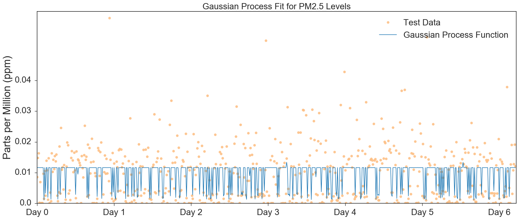
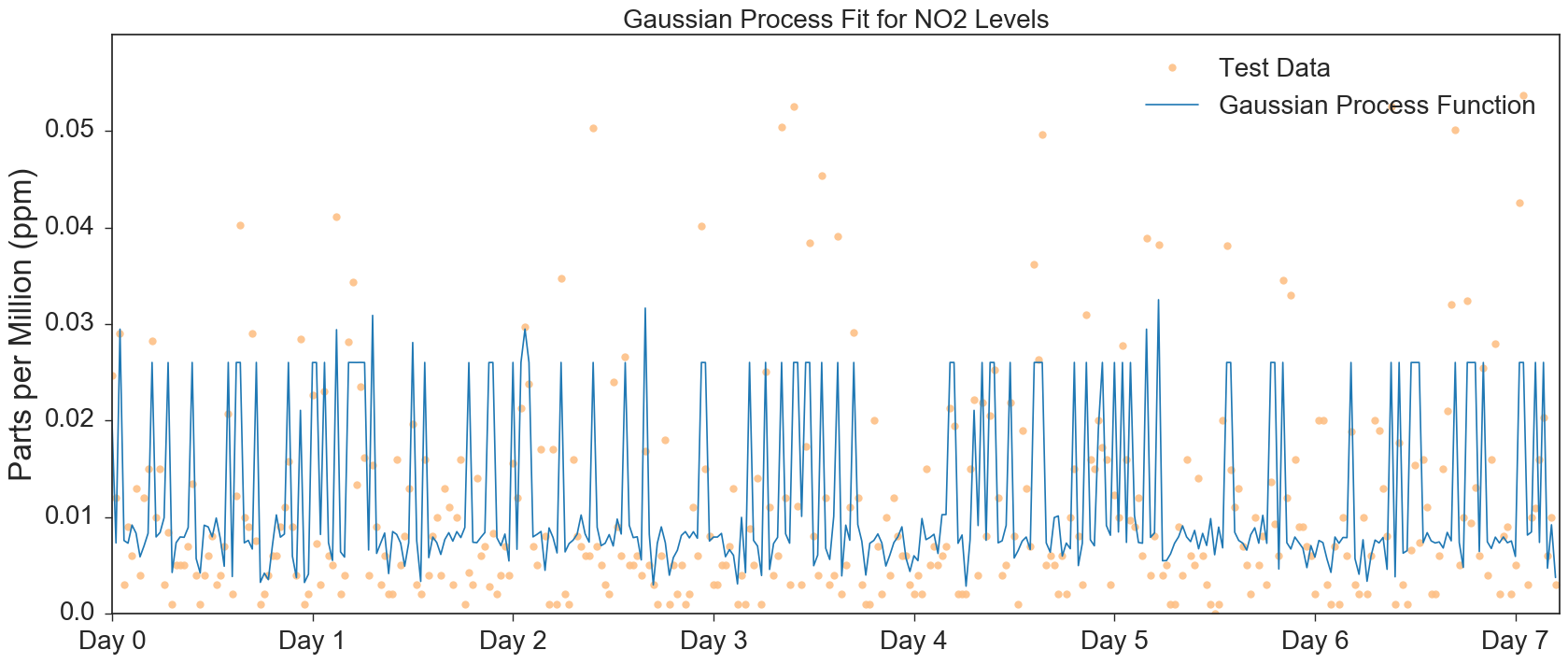
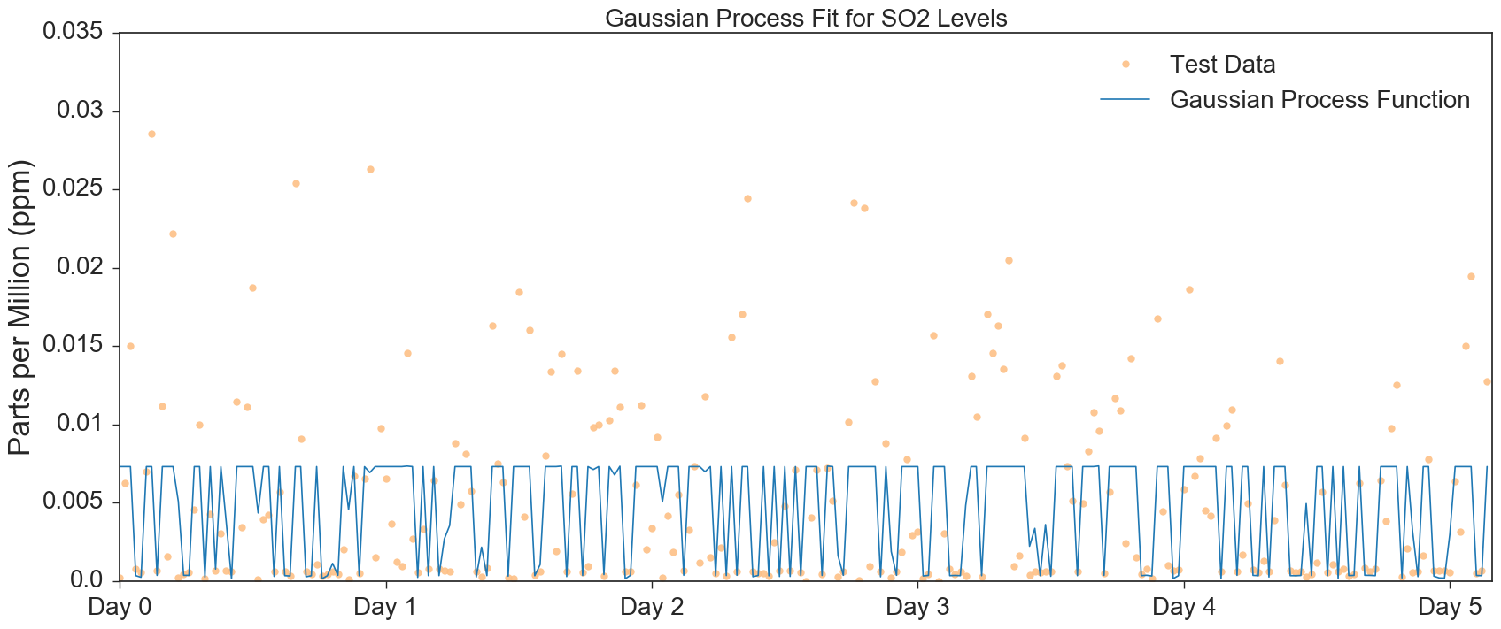
The temporal dependence of the pollution levels found by our Gaussian Process models are visualized in Figures 5 through 7.

VI. Analysis

Looking at Figure 6 and 7, for NO2 and PM2.5 respectively, we see that the Gaussian Processes are not fitting to higher concentration levels. Though we attempted to increase the amplitude of the Gaussian Process, the fit maintained its clipped appearance. The predicted levels of NO2 seems to experience significantly less clipping, hence its superior R2 values.

A common theme in all three of our Guassian Process models is that they did not perform significantly better than our LUR models, as we initially hypothesized (and as existing studies in literature would indicate). One possible explanation is that further feature engineering is required - in a number of studies in literature, significant features include variables absent from our model, e.g. distance from grid center or monitoring site to city center, total length of road segments contained in grid etc. Another compelling possibility explaining the poor performance of the Gaussian Process Model is that it mixes geospatial predictors extracted from the 1970’s and 80’s with dynamic predictors gathered from 2017. Given our limited time and computing resources, coupled with the difficulty of obtaining model ready data we were unable to gather sufficient geospatial and dynamic data from the same time period. Further data collection is our immediate future goal.

The primary goal for our web interface was to make data exploration and analysis an interactive and educational experience for all users. We wanted to implement a tour that would educate the user on the effects of air pollution and our research findings. The other setting in our interface is an interactive advanced view setting, which would include air pollutants in relation to health effects, visuals of the different geographical layers, and a time bar to show how pollution varies throughout the day. While we have successfully implemented the framework for most of the features in the advanced view button, the take a tour option still needs to be completed. We also need to add all of the desired layers and data to the advanced view, and change the way the data is visualized.

To date, our progress is as follows. We have set up the format of our interface. This includes assigning space allocated to the map, sidebar, and footer. We used CSS as our style-sheet for our interface. Here, we implemented the color scheme, the translucent sidebar and footer, and the two buttons (tour and advanced view). We have a fully functioning drop down menu, as well as a placeholder area for a small graph to show pollution over time when specific cells in the grid are hovered over. Lastly, we used D3.js, a Javascript library, to attach an interactive map that is drag-able and zoom-able, implement on-click effects, and create a interactive drop down menu on the advanced view button. Further steps will include adding more data layers, visualizing pollutant concentrations, implementing a trend line for Boston as a whole, and adding an interactive tour for new users.

VII. Conclusion

Air quality measurements, while not widely available or understandable, are crucial for understanding public health. Given that the average person is unaware of the air quality in the area they live, our main goal was to model the intraurban pollution variations in the Boston area and present this information to the public in a intuitive and engaging way. While there were time and resource constraints limiting the quality of the data collected, our models can be expanded upon to create better predictions in a variety of places. Our interface could also be generalized to fit a number of other cities and their data. Since Sulfur Dioxide, Nitrogen Dioxide, and Particulate Matter 2.5 can exacerbate cardiovascular and respiratory issues, it is crucial that the public have knowledge of areas to avoid and city-specific issues to be addressed. Ideally, our models (with up to date data and more parameters) would accurately predict criteria pollutant concentrations in each grid cell, thus areas with problematic concentrations could be appropriately researched efforts to reduce concentrations could me employed. Most importantly, the health layers will allow those with carcardiovascular or respiratory concerns to avoid high risk areas by assessing the temporal and spatial elements of the map.

VIII. Acknowledgements

Weiwei Pan, Harvard Institute for Applied Computational Science

Pavlos Protopapas, Harvard Institute for Applied Computational Science

Gary Adamkiewicz, Harvard T.H. Chan School of Public Health

Jaime Hart, Harvard T.H. Chan School of Public Health

IX. References

[1] Hasenfratz, David, Olga Saukh, Christoph Walser, Christoph Hueglin, Martin Fierz, Tabita Arn, Jan Beutel, and Lothar Thiele. ”Deriving High-resolution Urban Air Pollution Maps Using Mobile Sensor Nodes.” Pervasive and Mobile Computing 16 (2015): 268-85. Web.

[2] Hankey, Steve, Greg Lindsey, and Julian D. Marshall. ”Population- Level Exposure to Particulate Air Pollution during Active Travel: Planning for Low-Exposure, Health-Promoting Cities.” Environmental Health Perspectives 125.4 (2016): n. pag. Web.

[3] the American Heart Association. Circulation, vol. 121, no. 21, Oct. 2010, pp. 23312378., doi:10.1161/cir.0b013e3181dbece1.

[4] Brook, R. D. Air Pollution and Cardiovascular Disease: A Statement for Healthcare Professionals From the Expert Panel on Population and Prevention Science of the American Heart Association. Circulation, vol. 109, no. 21, Jan. 2004, pp. 26552671., doi:10.1161/01.cir.0000128587.30041.c8.

[5] Hamra, Ghassan B., et al. Outdoor Particulate Matter Exposure and Lung Cancer: A Systematic Review and Meta-Analysis. Environmental Health Perspectives, June 2014, doi:10.1289/ehp.1408092.

[6] Karner, Alex A., et al. Near-Roadway Air Quality: Synthesizing the Findings from Real-World Data. Environmental Science and Technology, vol. 44, no. 14, 2010, pp. 53345344., doi:10.1021/es100008x.

[7] US Environmental Protection Agency. Air Quality Criteria for Particulate Matter (October 2004). Available at: https://cfpub.epa.gov/ncea/ risk/recordisplay.cfm?deid=87903. Accessed July 26, 2017.

[8] US Environmental Protection Agency. Risk and Exposure Assessment to Support the Review of the SO2 Primary National Ambient Air Quality Standards: Final Report (July 2009). Available at: https://www3.epa.gov/ttn/naaqs/standards/so2/data/ 200908SO2REAFinalReport.pdf Accessed July 26, 2017.

[9] US Environmental Protection Agency. Risk and Exposure Assessment to Support the Review of the NO2 Primary National Ambient Air Quality Standard (November 2008). Available at: https://www3.epa.gov/ttn/naaqs/standards/nox/data/20081121 NO2 REA final.pdf Accessed July 26, 2017.

[10] Much of the information on the health impacts of our criteria pollutants came from conversations with Dr. Jaime Hart of the Harvard T.H. Chan School of Public Health.

[11] Satellite map images and air quality sensor locations were obtained from the Environmental Protection Agency (EPA) Interactive AirData Map. Web. 12 July 2017.

Report (PDF)